Top 80 Snowflake / BigQuery
interview questions
Warehouse architecture, partitioning, clustering and cost control. Open a question to read the answer.
01Explain Snowflake architecture storage compute in the context of Snowflake / BigQuery.
Snowflake separates storage from compute and puts a third layer, cloud services, on top of both. Data lives once in object storage (S3, Azure Blob, or GCS) as compressed, columnar micro-partitions; any number of independent compute clusters, called virtual warehouses, read that same data; and the cloud services layer handles authentication, metadata, query parsing and optimisation, transactions and result caching.
- Storage layer — immutable micro-partitions, encrypted, billed per compressed terabyte per month, shared by every warehouse.
- Compute layer — virtual warehouses of MPP nodes, each with local SSD cache; they can be created, resized, suspended and resumed independently and are billed in credits per second while running.
- Cloud services layer — the “brain”: metadata store, optimizer, security, and the 24-hour result cache. Mostly free unless it exceeds 10% of daily compute usage.
The diagram shows how several warehouses hit one copy of the data.
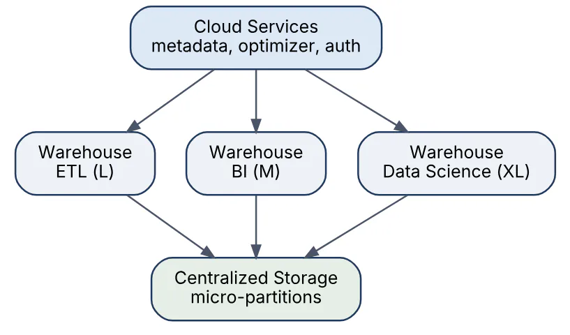
BigQuery’s equivalent is Dremel compute over Colossus storage joined by the Jupiter network, but the compute is fully serverless slots rather than user-managed warehouses.
02In a real project using Snowflake / BigQuery, how would you apply, test, or troubleshoot Snowflake architecture storage compute?
Apply. In a retail analytics platform I give each workload its own warehouse: LOAD_WH for the nightly ELT, BI_WH as a multi-cluster warehouse for Tableau, and DS_WH for ad hoc notebooks. All three read the same RAW and CURATED databases, so a heavy model-training query never slows the dashboards, and each team’s credits show up separately in WAREHOUSE_METERING_HISTORY. Auto-suspend is set to 60 seconds for the ELT warehouse and five minutes for BI so the result and local caches stay warm during office hours.
Test. I prove isolation by running a deliberately expensive cross join on DS_WH while a load test replays the top 50 dashboard queries against BI_WH; p95 latency on the BI side must not move. I also verify that resizing a warehouse mid-run does not corrupt in-flight statements and that a suspended warehouse resumes within the SLA.
Troubleshoot. The classic symptom is “the warehouse is slow” when the real cause is queuing: QUERY_HISTORY shows large queued_overload_time. The fix is more clusters, not a larger size. Conversely, heavy bytes_spilled_to_remote_storage means the warehouse is too small for the working set. For storage, unexpected growth usually traces back to Time Travel retention on a frequently rewritten table, visible in TABLE_STORAGE_METRICS.
The important caveat is that separation of storage and compute does not make compute free: an idle warehouse without auto-suspend bills every second.
03Explain virtual warehouses sizing in the context of Snowflake / BigQuery.
A virtual warehouse is a named cluster of compute nodes, and its size (XS, S, M, L, XL, 2XL up to 6XL) determines how many nodes it has. Each step up doubles the nodes, the memory, the local SSD cache and the credit rate: an XS burns 1 credit per hour, an S 2, an M 4, and so on to 512 for a 6XL. Billing is per second with a 60-second minimum each time the warehouse starts.
Sizing rules of thumb:
- Scale up (bigger size) when a single query is slow because it spills to disk or scans many partitions; a query that takes 10 minutes on an S should take roughly 5 on an M for the same credits.
- Scale out (multi-cluster warehouse, Enterprise edition) when many concurrent users cause queuing; extra clusters start and stop automatically between
MIN_CLUSTER_COUNTandMAX_CLUSTER_COUNT. - Set
AUTO_SUSPENDlow andAUTO_RESUME = TRUEso you pay only while queries run.
CREATE WAREHOUSE bi_wh
  WAREHOUSE_SIZE = 'MEDIUM'
  MIN_CLUSTER_COUNT = 1 MAX_CLUSTER_COUNT = 4
  SCALING_POLICY = 'STANDARD'
  AUTO_SUSPEND = 300 AUTO_RESUME = TRUE;
BigQuery has no warehouses to size; its analogue is choosing between on-demand pricing and a slot reservation with a baseline and autoscaling maximum.
04In a real project using Snowflake / BigQuery, how would you apply, test, or troubleshoot virtual warehouses sizing?
Apply. For a finance data mart I start every warehouse at XS or S and let evidence drive growth. The dbt transformation warehouse runs at L for 40 minutes a night because the big fact rebuilds spill at M; the Looker warehouse stays at M but is multi-cluster (1 to 3) because its problem is concurrency at 9 a.m., not single-query latency. A RESOURCE MONITOR on each warehouse notifies at 75% of the monthly quota and suspends at 100%.
Test. Sizing is an experiment: I run the same representative query set at two sizes with USE_CACHED_RESULT = FALSE, then compare elapsed time and credits from QUERY_HISTORY. If doubling the size halves the time, the query is compute-bound and the cost is neutral; if it only improves 20%, the smaller size wins. For multi-cluster settings I replay a concurrency peak with JMeter and watch WAREHOUSE_LOAD_HISTORY for avg_queued_load.
Troubleshoot. Users report random slowness at month end. QUERY_HISTORY shows queued_overload_time of several minutes while execution_time is normal, so I raise MAX_CLUSTER_COUNT rather than the size. The opposite case, a single dashboard query with gigabytes spilled to remote storage in the Query Profile, is solved by moving that workload to a larger warehouse or enabling the Query Acceleration Service.
Doubling warehouse size doubles cost per second, so an oversized warehouse serving tiny queries is the most common silent waste.
05Explain micro-partitions and pruning in the context of Snowflake / BigQuery.
Snowflake stores every table as a set of immutable micro-partitions, contiguous units of 50 to 500 MB of uncompressed data, stored columnar and compressed. For each micro-partition the cloud services layer keeps metadata: the min and max value of every column, the number of distinct values, null counts and the row count. Partitions are created automatically in insert order; nobody defines them.
Pruning is the optimizer’s use of that metadata to skip partitions. For WHERE order_date = '2026-03-01' it reads only partitions whose min/max range for order_date includes that day. Because columns are stored separately, it also prunes columns, reading only those the query references. Good pruning is why a filtered query on a 10 TB table can finish in seconds.
The diagram shows how min/max metadata lets a date filter skip most partitions.
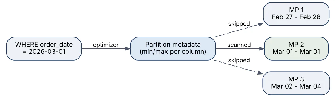
Pruning works well when data arrives roughly sorted on the filter column (dates in event tables) and poorly when the column is random (a UUID) or when the predicate wraps the column in a function the optimizer cannot push down, such as WHERE TO_CHAR(order_date, 'YYYY') = '2026'.
BigQuery’s equivalent is the Capacitor columnar format plus explicit table partitioning and block-level clustering metadata; Snowflake’s partitions are automatic, BigQuery’s partitions are declared.
06In a real project using Snowflake / BigQuery, how would you apply, test, or troubleshoot micro-partitions and pruning?
Apply. In an event pipeline landing 2 billion clickstream rows a month, I make sure loads arrive ordered by event_ts so each micro-partition covers a narrow time window. Downstream models always filter on event_ts with sargable predicates (event_ts >= :start AND event_ts < :end), never on DATE(event_ts). Where analysts also filter on tenant_id, I add a clustering key on (TO_DATE(event_ts), tenant_id).
Test. The Query Profile is the test harness. For each critical query I check the TableScan node: “Partitions scanned” versus “Partitions total”. A ratio near 1 means pruning failed. I keep this as a regression check by comparing partitions_scanned and partitions_total from QUERY_HISTORY after every schema or load change.
SELECT query_id, partitions_scanned, partitions_total,
       bytes_scanned / 1e9 AS gb_scanned
FROM   snowflake.account_usage.query_history
WHERE  query_tag = 'daily_sessions' AND start_time > DATEADD(day, -7, CURRENT_DATE)
ORDER  BY start_time DESC;
Troubleshoot. A query that used to take 20 seconds suddenly takes 4 minutes. The profile shows 100% of partitions scanned; the root cause was a backfill that reloaded two years of history in random order, destroying the natural date ordering. The fix was INSERT OVERWRITE ... ORDER BY event_ts to rewrite the table sorted, or enabling automatic clustering.
Pruning only helps with filters the optimizer can evaluate against min/max metadata; LIKE '%abc%' and function-wrapped columns always force a full scan.
07Explain clustering keys in the context of Snowflake / BigQuery.
A clustering key is one or more columns or expressions you declare on a Snowflake table so that Automatic Clustering keeps micro-partitions physically grouped by those values. It is an opt-in replacement for relying on natural insert order, and it exists purely to improve pruning on large tables (Snowflake suggests it only above roughly a terabyte).
Key points:
- Define with
ALTER TABLE t CLUSTER BY (TO_DATE(event_ts), region); low-cardinality or truncated expressions first, high-cardinality later. - A background serverless service re-sorts partitions as data arrives; it costs credits, reported in
AUTOMATIC_CLUSTERING_HISTORY, and can be paused withALTER TABLE ... SUSPEND RECLUSTER. SYSTEM$CLUSTERING_INFORMATION('t', '(col)')reports average depth and overlap; depth near 1 is ideal, high depth means many partitions overlap for the same value.- Clustering is worthless on columns you never filter or join on, and expensive on tables with constant random updates.
ALTER TABLE sales.fact_orders CLUSTER BY (TO_DATE(order_ts), store_id);
SELECT SYSTEM$CLUSTERING_INFORMATION('sales.fact_orders');
BigQuery’s CLUSTER BY (up to four columns) is the direct equivalent, but BigQuery re-clusters for free in the background and combines it with declared partitioning.
08In a real project using Snowflake / BigQuery, how would you apply, test, or troubleshoot clustering keys?
Apply. On a 30 TB telecom call-detail table queried almost always by call_date and subscriber_id, insert order gives good date pruning but nothing for subscriber lookups. I cluster on (call_date, subscriber_id) so the per-subscriber queries that drive the fraud dashboard prune on both. Smaller dimension tables stay unclustered; the cost of reclustering would exceed any benefit.
Test. Before committing, I clone the table (zero-copy), add the key to the clone, let Automatic Clustering finish, then run the top 20 queries against both with result caching off and compare partitions_scanned and elapsed time. I also compare credits_used from AUTOMATIC_CLUSTERING_HISTORY over a week against the compute saved; the key stays only if it pays for itself. SYSTEM$CLUSTERING_DEPTH is tracked daily in a monitoring table.
Troubleshoot. Two typical failures. First, clustering cost explodes: the table receives constant small updates that keep invalidating partitions, visible as a steady credit burn in AUTOMATIC_CLUSTERING_HISTORY. Fix by batching updates or clustering on a coarser expression such as DATE_TRUNC('month', call_date). Second, clustering shows good depth but queries still scan everything: the predicates use a different expression (subscriber_id::STRING) than the key, so the optimizer cannot match them.
The common mistake is clustering a high-cardinality column first; put the coarse column first so partitions form meaningful ranges.
09Explain Snowpipe ingestion in the context of Snowflake / BigQuery.
Snowpipe is Snowflake’s serverless, continuous file-loading service. A PIPE object wraps a COPY INTO statement; when new files land in a stage (S3, Azure Blob, GCS), Snowpipe loads them within minutes using Snowflake-managed compute, so no warehouse is needed and billing is per second of serverless compute plus a small per-file overhead.
Two trigger modes exist:
- Auto-ingest — cloud event notifications (S3 event to SQS, Azure Event Grid, GCS Pub/Sub) tell the pipe a file arrived.
- REST API — the producer calls
insertFileswith the file names, used when notifications are not available.
CREATE PIPE raw.orders_pipe AUTO_INGEST = TRUE AS
  COPY INTO raw.orders
  FROM @raw.orders_stage
  FILE_FORMAT = (TYPE = 'JSON');
The diagram shows the auto-ingest path from a file landing to rows in the table.

Snowpipe keeps load history per pipe for 14 days and skips files it has already loaded, so re-delivered notifications are harmless. Snowpipe Streaming is the row-level companion: an SDK or Kafka connector writes rows directly into a table with seconds of latency and no files at all.
BigQuery’s closest equivalents are Cloud Storage triggered load jobs (usually via Cloud Functions, Dataflow or the Data Transfer Service) for files, and the Storage Write API for streaming rows.
10In a real project using Snowflake / BigQuery, how would you apply, test, or troubleshoot Snowpipe ingestion?
Apply. For an IoT platform, devices publish to Kinesis Firehose, which writes gzipped JSON files of about 100 MB to S3 every five minutes. An auto-ingest pipe loads them into a VARIANT landing table; a stream and task downstream flatten the payload. File size matters: Snowpipe charges a per-file overhead, so I tune Firehose to avoid thousands of tiny files.
Test. In a staging account I drop a known set of files into the stage and poll SYSTEM$PIPE_STATUS('raw.telemetry_pipe') until pendingFileCount is zero, then assert the row count against the file manifest. COPY_HISTORY is queried for status <> 'Loaded' to catch partial loads. I also test the failure path by uploading a malformed file and checking that ON_ERROR = 'CONTINUE' behaves as expected and that the error rows appear in the history.
SELECT file_name, status, row_count, first_error_message
FROM TABLE(information_schema.copy_history(
  table_name => 'RAW.TELEMETRY',
  start_time => DATEADD(hour, -2, CURRENT_TIMESTAMP())));
Troubleshoot. Files land but nothing loads. The checklist: does SYSTEM$PIPE_STATUS show executionState = RUNNING? Is the S3 bucket notification pointing at the SQS ARN from SHOW PIPES (notification_channel)? Has the pipe been paused after an ownership change or 14 days of inactivity? Files with the same name as an already-loaded file are silently skipped; COPY_HISTORY reveals that too.
A notable limitation is that Snowpipe does not guarantee load order, so downstream logic must tolerate out-of-order arrival.
11Explain streams and tasks in the context of Snowflake / BigQuery.
A stream is a change-data-capture object on a table, view or external table. It records the delta (inserts, updates, deletes) since the last time it was consumed in a DML statement, exposing each changed row with METADATA$ACTION, METADATA$ISUPDATE and METADATA$ROW_ID. Reading the stream in a transaction that writes somewhere advances its offset; reading with a plain SELECT does not. Stream types are standard (all changes), append-only (inserts only) and insert-only (external tables).
A task is a scheduled unit of SQL, a stored procedure call or a Snowpark function. Tasks run on a user warehouse or serverless compute, on a SCHEDULE (minutes or CRON) or AFTER another task, which lets you build a DAG. The WHEN SYSTEM$STREAM_HAS_DATA('s') condition makes the task skip (free) when the stream is empty.
CREATE STREAM orders_stream ON TABLE raw.orders;

CREATE TASK merge_orders
  WAREHOUSE = etl_wh SCHEDULE = '5 MINUTE'
  WHEN SYSTEM$STREAM_HAS_DATA('orders_stream')
AS
  MERGE INTO curated.orders t USING orders_stream s ON t.id = s.id
  WHEN MATCHED AND s.METADATA$ACTION = 'DELETE' THEN DELETE
  WHEN MATCHED THEN UPDATE SET t.status = s.status
  WHEN NOT MATCHED THEN INSERT (id, status) VALUES (s.id, s.status);
The diagram shows how a stream feeds a task that merges changes downstream.

BigQuery’s equivalents are the CHANGES / APPENDS change-history functions plus scheduled queries, though they are less tightly coupled than a stream-task pair.
12In a real project using Snowflake / BigQuery, how would you apply, test, or troubleshoot streams and tasks?
Apply. In a subscription billing warehouse, Snowpipe lands raw invoice events; an append-only stream on the landing table feeds a root task that runs every ten minutes only when the stream has data, merges into a dim_customer SCD2 table, and a child task (AFTER) rebuilds the revenue aggregate. The root task is serverless so there is no warehouse to keep warm, and the whole DAG is owned by a dedicated role with EXECUTE TASK privilege.
Test. Unit testing a task means calling EXECUTE TASK merge_invoices on demand in a test schema, then asserting the target contents and that SELECT COUNT(*) FROM invoice_stream returns zero. I test idempotency by running the task twice with no new data and confirming the aggregate is unchanged. TASK_HISTORY is checked for state, scheduled_time versus completed_time drift, and error messages.
Troubleshoot. The two production incidents I see most often are staleness and silent skips. A stream becomes stale when it is not consumed within the table’s data retention period (extended up to 14 days by default); SHOW STREAMS shows stale = true and the fix is recreating the stream and backfilling. Silent skips happen when a task is created but never RESUMEd, or when the owning role loses the warehouse USAGE grant; TASK_HISTORY shows SKIPPED or a permission error.
One trap: a MERGE that reads a stream but fails mid-way rolls back and leaves the offset untouched, so retries are safe, but a successful SELECT INTO from the same stream in a separate transaction consumes it for everyone.
13Explain Time Travel and Fail-safe in the context of Snowflake / BigQuery.
Time Travel lets you query, clone or restore data as it existed at any point within a table’s retention period. Because micro-partitions are immutable, an update simply writes new partitions and the old ones are kept for the retention window. Retention is DATA_RETENTION_TIME_IN_DAYS: 1 day by default and maximum on Standard edition, up to 90 days on Enterprise and above; transient and temporary tables are capped at 1 day.
SELECT * FROM orders AT (TIMESTAMP => '2026-10-01 08:00:00'::TIMESTAMP_LTZ);
SELECT * FROM orders BEFORE (STATEMENT => '01b2c3d4-...');
UNDROP TABLE orders;
CREATE TABLE orders_restored CLONE orders AT (OFFSET => -3600);
The diagram shows how data moves through the two recovery windows before it is purged.

Fail-safe begins when Time Travel ends: a fixed, non-configurable 7 days during which only Snowflake Support can recover data, intended for disaster recovery rather than self-service. Transient tables have no Fail-safe, which is why they are cheaper for staging data. Both periods count toward storage billing, so a table rewritten daily with 90-day retention stores roughly 90 copies of its changed partitions.
BigQuery has the same two-stage model: a configurable 2 to 7 day time travel window queried with FOR SYSTEM_TIME AS OF, followed by a 7-day fail-safe that also requires Google support to use.
14In a real project using Snowflake / BigQuery, how would you apply, test, or troubleshoot Time Travel and Fail-safe?
Apply. In a healthcare warehouse I set DATA_RETENTION_TIME_IN_DAYS = 30 on the curated schema so analysts can reproduce any report from the past month, 1 day on the raw landing schema, and make all staging tables TRANSIENT to avoid Fail-safe storage. Every dbt run records its query_id in an audit table, so a bad deployment can be reverted with CREATE OR REPLACE TABLE fact_claims CLONE fact_claims BEFORE (STATEMENT => :bad_query_id) in seconds instead of a multi-hour reload.
Test. Recovery is rehearsed quarterly: a runbook drops a non-critical table, confirms UNDROP works, then restores a table to a timestamp and diff-checks row counts and checksums against a known snapshot. I also test the storage impact by loading a churned table at 1-day and 30-day retention and comparing TABLE_STORAGE_METRICS.TIME_TRAVEL_BYTES.
Troubleshoot. Two recurring issues. “Time Travel data is not available” errors mean the requested point is outside retention or the table was recreated with CREATE OR REPLACE, which starts a new object; the old one is reachable only via UNDROP after renaming the new one. A storage bill that doubles overnight is usually a large table switched to high retention plus a full daily rewrite; TABLE_STORAGE_METRICS separates active, Time Travel and Fail-safe bytes and points to the offender.
The important limitation is that Fail-safe is not a backup strategy: recovery is manual, slow and not guaranteed to meet an RTO, so critical datasets still need scheduled clones or replication.
15Explain zero copy cloning in the context of Snowflake / BigQuery.
Zero-copy cloning creates a new table, schema or database that is a complete, writable copy of the source at a point in time, without copying any data. Because micro-partitions are immutable, the clone simply receives its own metadata pointing to the same partitions. The operation takes seconds regardless of size and costs nothing in storage until either side changes: new or modified partitions are owned by whichever object wrote them, and only those are billed.
CREATE DATABASE analytics_dev CLONE analytics;
CREATE TABLE orders_backup CLONE orders AT (OFFSET => -86400);
Characteristics worth stating in an interview:
- Clones are independent objects; writes to one never affect the other.
- Can be combined with Time Travel to clone the state at a past moment.
- Grants on the cloned object itself are not copied by default (child objects’ grants are); use
COPY GRANTSwhere supported. - Internal stages, pipes referencing internal stages and external tables are not cloned.
Typical uses are dev/test environments from production, pre-deployment backups, and A/B testing of clustering keys. BigQuery offers the same idea with CREATE TABLE ... CLONE (writable, billed only on the delta) and read-only snapshots for backups.
16In a real project using Snowflake / BigQuery, how would you apply, test, or troubleshoot zero copy cloning?
Apply. Every CI pipeline for our dbt project clones the production ANALYTICS database into ANALYTICS_PR_<number>, runs the changed models and their tests against real data volumes, then drops the clone. Before each production release a task runs CREATE SCHEMA curated_backup_<date> CLONE curated so rollback is a rename. Developers also get a personal clone of a 5 TB database in under a minute, something a physical copy could never deliver.
Test. The main thing to verify is isolation and grants. A test suite writes to the clone and asserts the production row count is unchanged, then checks SHOW GRANTS ON TABLE to confirm the service role lost no privileges. For the backup clone, I validate restoration by swapping it in on a staging account with ALTER TABLE ... SWAP WITH and running the regression dashboard queries.
Troubleshoot. Clones that mysteriously cost money: TABLE_STORAGE_METRICS shows ACTIVE_BYTES growing on long-lived dev clones because developers rebuilt large tables inside them, and the production side rewrote its partitions too, so neither shares anything any more. The fix is an expiry task that drops clones older than seven days. Another frequent ticket is “my clone lost access”: the clone of a schema does not inherit grants on the schema itself, so the deployment script must re-grant USAGE.
A trade-off to remember is that cloning a database does not clone its pipes with auto-ingest enabled in a running state; they come over paused and must be reviewed before resuming to avoid double loads.
17Explain secure data sharing in the context of Snowflake / BigQuery.
Secure Data Sharing lets a provider account expose tables, secure views, secure UDFs and dynamic tables to consumer accounts without copying or moving any data. The provider creates a SHARE, grants object privileges to it, and adds consumer account identifiers; the consumer creates a read-only database from the share and queries it with its own compute. The data remains in the provider’s storage, so the consumer always sees the current version and the provider pays storage while the consumer pays compute.
CREATE SHARE sales_share;
GRANT USAGE ON DATABASE sales TO SHARE sales_share;
GRANT USAGE ON SCHEMA sales.public TO SHARE sales_share;
GRANT SELECT ON VIEW sales.public.v_orders_partner TO SHARE sales_share;
ALTER SHARE sales_share ADD ACCOUNTS = partner_org.partner_acct;
The diagram shows that the consumer queries the provider’s storage through a read-only database, with no copy.
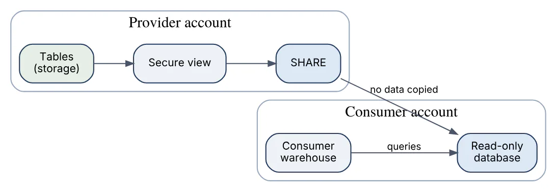
Important mechanics:
- Shares are intra-region by default; cross-region or cross-cloud sharing requires replicating the database to the target region first.
- Reader accounts let the provider share with organisations that are not Snowflake customers, with the provider paying their compute.
- Listings and the Snowflake Marketplace wrap shares with discovery, terms and usage metrics.
- Secure views are mandatory for row filtering so consumers cannot infer hidden data through the optimizer.
BigQuery’s equivalent is BigQuery sharing (formerly Analytics Hub) with listings and linked datasets, plus authorized views and datasets for finer-grained read-only exposure.
18In a real project using Snowflake / BigQuery, how would you apply, test, or troubleshoot secure data sharing?
Apply. A logistics company shares shipment status with 40 carriers. Each carrier gets the same SHARE, but the shared object is a secure view filtered by CURRENT_ACCOUNT() against a mapping table, so one share serves all carriers with row-level isolation. Carriers without Snowflake receive reader accounts governed by a resource monitor that caps their compute at 20 credits per month. The share is published as a private listing so the legal terms and contact details travel with it.
Test. From a test consumer account I assert three things: the view returns only that account’s rows, SELECT COUNT(*) on a direct reference to the base table fails with an authorization error, and attempts to clone or Time Travel the shared table are rejected. I also test change propagation by adding a column in the provider and confirming the consumer sees it only after the view is recreated and re-granted.
Troubleshoot. “Share not visible” is almost always a region mismatch: the consumer account lives in a different region, so I set up database replication to a provider account there and share from the replica. The second common fault is a secure view referencing an object the share does not have USAGE / SELECT on, which surfaces as a permission error for the consumer; SHOW GRANTS TO SHARE lists what is missing.
The main limitation is that consumers cannot modify or re-share the data, and provider-side CREATE OR REPLACE of a shared view silently drops it from the share.
19Explain Snowflake RBAC in the context of Snowflake / BigQuery.
Snowflake uses role-based access control layered on discretionary ownership: every object has exactly one owning role, privileges are granted to roles, roles are granted to other roles or to users, and a user operates under one primary role plus optional secondary roles. There are no direct user- to-object grants.
The system roles form the top of the hierarchy: ACCOUNTADMIN (everything; use sparingly), SECURITYADMIN (manages grants), USERADMIN (users and roles), SYSADMIN (creates and owns databases and warehouses) and PUBLIC. Best practice is to create functional roles (ANALYST, ETL_WRITER) and access roles per schema (SALES_READ, SALES_RW), grant access roles to functional roles, and roll everything up to SYSADMIN so admins can see all objects.
CREATE ROLE sales_read;
GRANT USAGE ON DATABASE sales TO ROLE sales_read;
GRANT USAGE ON ALL SCHEMAS IN DATABASE sales TO ROLE sales_read;
GRANT SELECT ON ALL TABLES IN SCHEMA sales.public TO ROLE sales_read;
GRANT SELECT ON FUTURE TABLES IN SCHEMA sales.public TO ROLE sales_read;
GRANT ROLE sales_read TO ROLE analyst;
GRANT ROLE analyst TO USER priya;
Future grants keep new tables covered automatically. Database roles and managed access schemas (WITH MANAGED ACCESS) centralise grant control with the schema owner. This TB diagram shows a typical hierarchy.
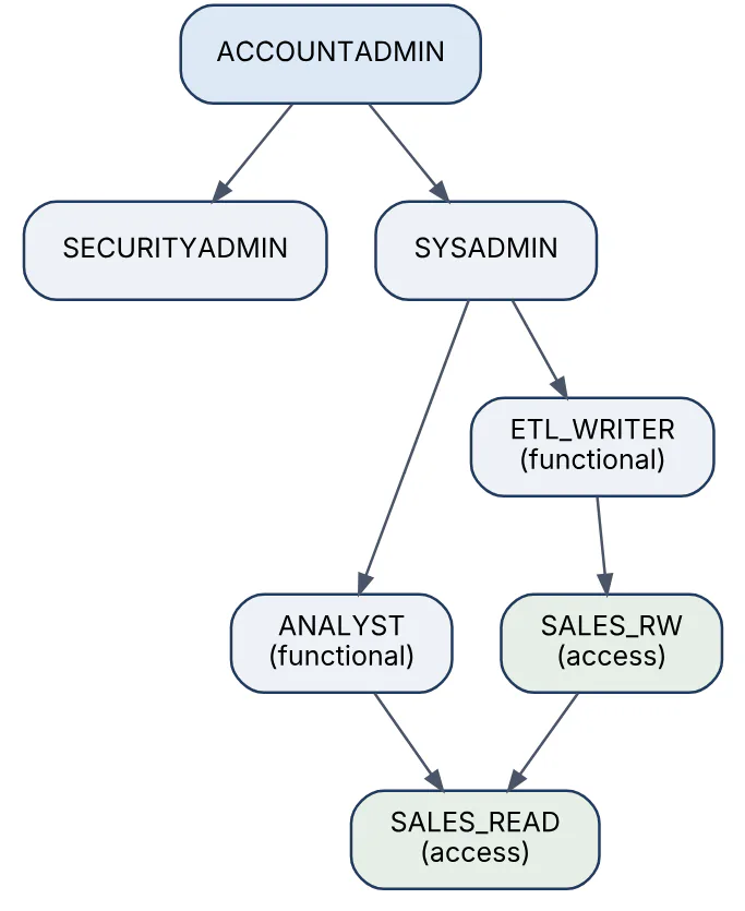
BigQuery instead uses Cloud IAM: predefined or custom roles bound to principals at project, dataset, table or row level, with no ownership chain.
20In a real project using Snowflake / BigQuery, how would you apply, test, or troubleshoot Snowflake RBAC?
Apply. For a multi-team platform I manage the whole role tree in Terraform: one access role pair (_R, _RW) per schema with future grants, functional roles per team, and a DEPLOY role that owns everything created by CI so ownership never lands on a human. Users authenticate through Okta SCIM, which maps groups to functional roles, so onboarding is a group change rather than a GRANT. Service accounts use key-pair auth with their default role pinned.
Test. A nightly test logs in as a synthetic user per functional role and runs a matrix of statements: SELECT on each schema, INSERT on write schemas, CREATE TABLE where allowed, and expects explicit Insufficient privileges errors elsewhere. Drift is detected by diffing SHOW GRANTS output against the Terraform state, and the test fails if any user holds ACCOUNTADMIN outside the break-glass list.
Troubleshoot. “Object does not exist or not authorized” is the standard symptom; it hides three causes. First, missing USAGE on the database or schema even though SELECT on the table is present. Second, the table was created after the role was set up and no future grant exists. Third, the user ran with the wrong primary role; SELECT CURRENT_ROLE() and USE SECONDARY ROLES ALL settle that quickly. Ownership tangles, where a developer’s personal role owns a production table and they leave, are fixed with GRANT OWNERSHIP ... COPY CURRENT GRANTS.
A frequent mistake is granting privileges to PUBLIC for convenience, which effectively gives every user in the account access.
21Explain Snowflake query profile in the context of Snowflake / BigQuery.
The Query Profile is Snowflake’s visual execution plan with runtime statistics, available in Snowsight for any query in history. It shows the operator tree (TableScan, Filter, Join, Aggregate, Sort, Result) with the percentage of total time each node consumed, the rows flowing between nodes, and a statistics panel that is where most diagnoses happen:
- Pruning — partitions scanned versus partitions total; close to total means filters are not pruning.
- Spilling — bytes spilled to local storage (SSD, tolerable) and to remote storage (object storage, slow); remote spilling means the warehouse lacks memory.
- Join explosion — a Join node emitting far more rows than either input signals a missing or non-unique join key.
- Network and I/O — bytes sent over the network, percentage scanned from cache.
- Queued time versus execution time, exposing concurrency problems.
The same data is available programmatically through GET_QUERY_OPERATOR_STATS(query_id) for automated analysis, and EXPLAIN gives the plan without running the query. BigQuery’s equivalent is the “Execution details” tab (query stages with wait, read, compute and write time) plus INFORMATION_SCHEMA.JOBS fields such as total_slot_ms and total_bytes_processed.
22In a real project using Snowflake / BigQuery, how would you apply, test, or troubleshoot Snowflake query profile?
Apply. Every dbt model carries a query_tag, so when the nightly run exceeds its time budget I filter QUERY_HISTORY by tag, sort by total_elapsed_time, and open the profile of the top offenders. Review of the profile is also part of our pull-request checklist for any model touching a fact table: the reviewer must paste the partitions scanned/total ratio and the spill figures.
Test. Performance tests capture a baseline from GET_QUERY_OPERATOR_STATS for critical queries and fail the pipeline if bytes_spilled_to_remote_storage becomes non-zero or partitions_scanned grows more than 20% without a corresponding growth in data. This turns the profile into a regression test rather than a tool you open after an outage.
SELECT operator_type, operator_statistics:pruning:partitions_scanned AS scanned,
       operator_statistics:pruning:partitions_total AS total,
       execution_time_breakdown:overall_percentage AS pct
FROM TABLE(GET_QUERY_OPERATOR_STATS(LAST_QUERY_ID()))
WHERE operator_type = 'TableScan';
Troubleshoot. A report query ballooned from 30 seconds to 25 minutes. The profile showed a Join node producing 40 billion rows from two inputs of 10 million each: a many-to-many join on customer_id after a source system started emitting duplicate customer records. Deduplicating with QUALIFY ROW_NUMBER() OVER (...) = 1 upstream restored the runtime. In another case, heavy remote spilling on an aggregate was fixed by moving the job to a larger warehouse, which was cheaper than the slow run.
The caveat is that the profile reflects a single execution; cache state and concurrent load change the numbers, so compare runs with USE_CACHED_RESULT = FALSE.
23Explain Snowflake cost optimization in the context of Snowflake / BigQuery.
Snowflake bills three things: compute (credits per second of warehouse or serverless usage), storage (per compressed TB per month, including Time Travel and Fail-safe) and data transfer (egress across regions or clouds). Compute dominates nearly every bill, so optimisation starts there.
Main levers:
- Auto-suspend and auto-resume — 60 seconds for batch warehouses; longer only when cache hits justify it.
- Right-size per workload — separate warehouses per team, start small, scale up only for spilling, scale out only for queuing.
- Resource monitors — credit quotas with notify and suspend actions per warehouse or account.
- Reduce scanned data — pruning-friendly predicates, clustering where it pays, avoiding
SELECT *. - Storage hygiene — transient tables for staging, short Time Travel on volatile tables, drop forgotten clones.
- Serverless features — Snowpipe, tasks and automatic clustering have their own meters; review them in
METERING_DAILY_HISTORY. - Visibility —
WAREHOUSE_METERING_HISTORY,QUERY_ATTRIBUTION_HISTORY(per-query credits) and query tags to chargeback by team.
Budgets (account-level spending limits with alerts) complement resource monitors. BigQuery’s cost model is different: on-demand bills bytes scanned, editions bill slot-hours, so the equivalent levers are partition filters, clustering, maximum_bytes_billed, and choosing the right edition and autoscaling ceiling.
24In a real project using Snowflake / BigQuery, how would you apply, test, or troubleshoot Snowflake cost optimization?
Apply. On a platform burning 60,000 credits a year I introduced three habits. Each warehouse received a resource monitor with a monthly quota and a 1-minute auto-suspend; every job sets QUERY_TAG = '<team>:<pipeline>'; and a weekly Snowsight dashboard built on QUERY_ATTRIBUTION_HISTORY ranks the ten costliest queries by team. Staging schemas became transient with 0-day retention, which alone cut storage 35%.
Test. Optimisation changes are measured, not assumed. Before and after each change I compare seven days of WAREHOUSE_METERING_HISTORY normalised by rows processed, so a drop in traffic is not mistaken for savings. A unit test on the Terraform module asserts that no warehouse is created without AUTO_SUSPEND <= 300 and a monitor attached.
SELECT warehouse_name, SUM(credits_used) AS credits
FROM snowflake.account_usage.warehouse_metering_history
WHERE start_time >= DATEADD(day, -7, CURRENT_DATE)
GROUP BY 1 ORDER BY 2 DESC;
Troubleshoot. A sudden 3x credit spike with flat query volume pointed to a warehouse whose auto-suspend had been set to NULL during an incident and never restored; WAREHOUSE_EVENTS_HISTORY showed it running 24 hours a day. A slower creep came from automatic clustering on a table with constant upserts, visible in AUTOMATIC_CLUSTERING_HISTORY; suspending reclustering and batching updates removed it.
The trade-off everyone forgets: aggressive auto-suspend evicts the local SSD cache, so interactive BI warehouses may be cheaper with a five-minute timeout than with sixty seconds.
25Explain Snowflake semi-structured VARIANT in the context of Snowflake / BigQuery.
VARIANT is Snowflake’s universal semi-structured type: a column that can hold any JSON, Avro, ORC, Parquet or XML value, including nested objects and arrays, up to 128 MB uncompressed per value. Internally Snowflake shreds the data into columnar sub-columns with statistics, so queries on common paths are nearly as fast as on native columns, while rare or heterogeneous keys are kept in the raw form. OBJECT and ARRAY are the typed cousins.
Access uses path notation with casting:
SELECT payload:customer.id::NUMBER       AS customer_id,
       payload:customer.email::STRING    AS email,
       f.value:sku::STRING               AS sku,
       f.value:qty::INT                  AS qty
FROM raw.orders,
     LATERAL FLATTEN(input => payload:items) f
WHERE payload:status::STRING = 'PAID';
FLATTEN turns arrays into rows; PARSE_JSON, OBJECT_CONSTRUCT and TRY_CAST handle construction and safe conversion. INFER_SCHEMA and schema evolution on COPY let you promote stable keys into real columns later. Keys with mixed types across rows defeat the columnar shredding and should be cast or normalised early.
BigQuery’s equivalent is the native JSON type (with JSON_VALUE, JSON_QUERY and the . accessor), alongside its STRUCT and ARRAY types for strongly typed nesting.
26In a real project using Snowflake / BigQuery, how would you apply, test, or troubleshoot Snowflake semi-structured VARIANT?
Apply. For a marketplace ingesting webhooks from a dozen payment providers, each with a different schema, the landing table is (received_at, provider, payload VARIANT). A task reads a stream on it and projects a stable contract (amount, currency, status) into a typed table, keeping the raw payload beside it for audit. New provider fields cost nothing until an analyst needs them, and payload:status queries still prune well because the key is present in every row.
Test. Data contract tests run on every batch: a view asserts TYPEOF(payload:amount) = 'DECIMAL' for 100% of rows, that payload:items is an ARRAY, and that TRY_TO_NUMBER(payload:amount::STRING) never returns NULL where the raw value is present. A Great Expectations suite compares the flattened row count against SUM(ARRAY_SIZE(payload:items)) so no line items are lost.
Troubleshoot. A query filtering on payload:event_type suddenly scanned every partition. The cause was a provider that started sending the key as eventType; Snowflake path access is case-sensitive, so half the rows returned NULL and the column statistics became useless. Normalising keys with OBJECT_CONSTRUCT_KEEP_NULL and lower-casing at load fixed it. Another incident was a VARIANT column storing numbers as strings in some rows, which made ::NUMBER casts fail with “Numeric value is not recognized”; TRY_CAST plus a quarantine table isolated the bad rows.
The important limitation is that nested-path filters are only as prunable as the data is homogeneous; heavily polymorphic payloads belong in typed columns sooner rather than later.
27Explain Snowpark transformations in the context of Snowflake / BigQuery.
Snowpark is Snowflake’s developer framework for writing data transformations in Python, Scala or Java that execute inside Snowflake rather than on an external cluster. The core is a lazily evaluated DataFrame API: each operation (filter, join, group_by, with_column) builds a logical plan that is compiled into a single SQL statement and executed on a virtual warehouse when an action (collect, show, save_as_table) is called. No data leaves Snowflake unless you ask for it.
from snowflake.snowpark import Session
from snowflake.snowpark.functions import col, sum as sum_

session = Session.builder.configs(conn_params).create()
orders = session.table("raw.orders").filter(col("status") == "PAID")
daily = (orders.with_column("order_day", col("order_ts").cast("date"))
               .group_by("order_day", "region")
               .agg(sum_("amount").alias("revenue")))
daily.write.mode("overwrite").save_as_table("curated.daily_revenue")
Beyond DataFrames, Snowpark lets you register Python UDFs, vectorised UDFs (pandas batches), UDTFs and stored procedures that run in a sandboxed Python runtime with Anaconda packages, and schedule them with tasks. Use it when logic is awkward in SQL (custom parsing, ML scoring, loops over metadata) while keeping the pushdown benefits of the engine.
BigQuery’s equivalents are BigQuery DataFrames (the bigframes pandas-compatible library that compiles to SQL), Python UDFs, and Apache Spark stored procedures.
28In a real project using Snowflake / BigQuery, how would you apply, test, or troubleshoot Snowpark transformations?
Apply. In a fraud-scoring pipeline the feature engineering is plain SQL, but the scoring step calls a scikit-learn model. I package the model into a stage, register a vectorised Python UDF that loads it once per batch, and call it from a Snowpark DataFrame in a stored procedure scheduled by a task. Everything runs on the warehouse, so the data never crosses the network and the pipeline needs no Airflow worker with Python dependencies.
Test. Snowpark code is Python, so it gets pytest. Pure transformations are tested with the local testing framework (Session.builder.config("local_testing", True)), which runs DataFrame logic without a connection; integration tests execute against a cloned schema and compare daily.to_pandas() with a hand-computed expectation. UDFs are unit-tested as ordinary functions before registration, and the generated SQL (df.queries) is reviewed to make sure filters pushed down rather than pulling data to the client.
Troubleshoot. The most common problem is accidental data pull: a developer calls to_pandas() on 200 million rows and the client runs out of memory. Review of df.queries and insisting on save_as_table for large outputs fixes it. The second is UDF slowness; the Query Profile shows a Python UDF node dominating because the model was being loaded per row instead of once in the handler’s initialisation, or because the UDF was scalar rather than vectorised. Package conflicts surface as “package not found in Anaconda channel”; pinning versions in session.add_packages resolves them.
One consideration: Snowpark compute is still warehouse credits, so a tight Python loop issuing many small statements can cost more than one set-based SQL statement.
29Explain Snowflake dynamic tables in the context of Snowflake / BigQuery.
A dynamic table is a table defined by a query that Snowflake keeps up to date automatically. Instead of writing a stream, a task and a MERGE, you declare the desired result and a TARGET_LAG; Snowflake tracks changes in the base tables and refreshes the dynamic table, incrementally where the query shape allows it and with a full refresh otherwise. Dynamic tables reached general availability in 2024.
CREATE DYNAMIC TABLE curated.daily_revenue
  TARGET_LAG = '10 minutes'
  WAREHOUSE = etl_wh
AS
SELECT order_ts::DATE AS order_day, region, SUM(amount) AS revenue
FROM   raw.orders
WHERE  status = 'PAID'
GROUP  BY 1, 2;
Key behaviours:
TARGET_LAG = DOWNSTREAMlets a table refresh only when a dependent dynamic table needs it, forming a pipeline DAG with one lag setting at the end.REFRESH_MODEcan beAUTO,INCREMENTALorFULL;SHOW DYNAMIC TABLESreveals which mode was chosen and why incremental was rejected (non-deterministic functions, some window patterns).- Monitoring lives in
DYNAMIC_TABLE_REFRESH_HISTORYand the Snowsight graph view. - They are read-only; you cannot DML into them, and they cannot use Time Travel beyond the refresh history.
BigQuery’s closest equivalent is a materialized view with max_staleness or, for arbitrary SQL, a scheduled query writing to a table; dynamic tables sit between the two because they allow joins and nesting while still refreshing automatically.
30In a real project using Snowflake / BigQuery, how would you apply, test, or troubleshoot Snowflake dynamic tables?
Apply. For a near-real-time order dashboard I replaced four stream-task pairs with a chain of dynamic tables: stg_orders (cleaned, DOWNSTREAM lag) feeds fct_orders (joined with customers, DOWNSTREAM) which feeds agg_hourly_sales with TARGET_LAG = '5 minutes'. One lag setting at the leaf drives the whole chain, and the refresh graph in Snowsight replaces hand-written orchestration. Slowly changing lookups remain regular tables because they do not need lag guarantees.
Test. Correctness is tested by comparing the dynamic table with a plain CREATE TABLE AS of the same query after forcing ALTER DYNAMIC TABLE ... REFRESH; row counts and a hash of the sorted output must match. I also verify the chosen refresh mode with SHOW DYNAMIC TABLES and fail the deployment if a table meant to be incremental reports FULL, since that silently multiplies cost. Lag compliance is asserted from DYNAMIC_TABLE_REFRESH_HISTORY in staging under a synthetic write load.
Troubleshoot. A dynamic table stopped refreshing: SHOW DYNAMIC TABLES shows scheduling_state = SUSPENDED after five consecutive failures, and DYNAMIC_TABLE_REFRESH_HISTORY carries the error, typically a dropped column in a source table. Fix the query and ALTER DYNAMIC TABLE ... RESUME. A cost spike traced to one table falling back to full refresh because someone added CURRENT_TIMESTAMP() to the select list; replacing it with a source column restored incremental mode.
The important consideration is that target lag is a goal, not an SLA: under warehouse contention or a long-running refresh the actual lag can exceed it, so alert on data_timestamp age.
31Explain BigQuery serverless architecture in the context of Snowflake / BigQuery.
BigQuery is a fully serverless data warehouse: there is no cluster, warehouse or instance to create. Storage and compute are separate services connected by Google’s internal network. Tables are stored in Colossus, Google’s distributed file system, in the columnar Capacitor format, and replicated across zones within the chosen region. Queries run on Dremel, a multi-level tree of workers that splits each query into stages, and the shuffle tier moves intermediate results between stages in memory.
Compute is measured in slots, virtual CPUs with memory, allocated to a query dynamically for its duration. With on-demand pricing a project draws from a shared pool (up to 2,000 concurrent slots by default) and pays per byte scanned; with editions you reserve slot capacity and pay per slot-hour. Either way, the user never sizes, starts or stops anything. The flow below shows the moving parts.

Compared with Snowflake, where you choose warehouse sizes and pay per second they run, BigQuery removes capacity decisions entirely and shifts cost control to bytes processed or slot reservations.
32In a real project using Snowflake / BigQuery, how would you apply, test, or troubleshoot BigQuery serverless architecture?
Apply. A media company’s event warehouse receives spiky load: nothing overnight, thousands of dashboard queries during morning news. Serverless fits that shape. I keep ad hoc analysts on on-demand pricing with a per-user daily byte quota, and put the Looker service account and scheduled pipelines in an Enterprise edition reservation with a 100-slot baseline and autoscaling to 500, so predictable workloads have predictable cost and unpredictable ones cannot run away.
Test. Because there is nothing to provision, testing concentrates on behaviour under concurrency and on cost guards. A load test fires 200 simultaneous dashboard queries and I inspect INFORMATION_SCHEMA.JOBS_TIMELINE for slot contention and queue time. Cost tests run each pipeline query with --dry_run to assert total_bytes_processed stays below a budget, and maximum_bytes_billed is set on every scheduled job so a regression fails rather than bills.
Troubleshoot. “Query was slow today but fast yesterday” on on-demand usually means the shared pool was busy; JOBS_TIMELINE shows period_slot_ms far below what the query wanted. Moving that workload to a reservation fixes it. Another classic symptom is Resources exceeded during query execution, which is a single stage (often a huge ORDER BY without LIMIT or a skewed join key) overflowing shuffle memory; rewriting to avoid the global sort or pre-aggregating the skewed key resolves it.
The consideration to state is that serverless hides capacity but not cost: an unfiltered SELECT * on a 50 TB table is a legitimate, instantly executed, very expensive query.
33Explain BigQuery slots and reservations in the context of Snowflake / BigQuery.
A slot is BigQuery’s unit of compute: one virtual CPU with attached memory that works on one stage of a query at a time. Every query is broken into stages, and each stage is spread over as many slots as are available and useful; a complex query may use thousands of slot-seconds, and total_slot_ms in INFORMATION_SCHEMA.JOBS records exactly how many.
How slots are obtained:
| Model | Capacity | Billing | Best for |
|---|---|---|---|
| On-demand | Shared pool, soft cap of 2,000 slots per project | Per TiB scanned (1 TiB free monthly) | Ad hoc, low volume |
| Editions autoscaling | Baseline plus autoscale up to a max, in 50-slot steps | Per slot-hour while allocated | Steady pipelines, BI |
| Commitments | 1-year or 3-year slot commitments | Discounted slot-hour | Large, constant workloads |
Reservations are created in the admin project and then assigned to projects, folders or the whole organisation, optionally by job type (QUERY, PIPELINE, ML_EXTERNAL). Idle slots in one reservation are shared with others under the same admin project unless ignore_idle_slots is set. Editions (Standard, Enterprise, Enterprise Plus) govern which features a reservation unlocks, such as materialized view smart tuning or cross-region replication.
The diagram shows how a query’s stages run on a reservation’s baseline and autoscaled slots.
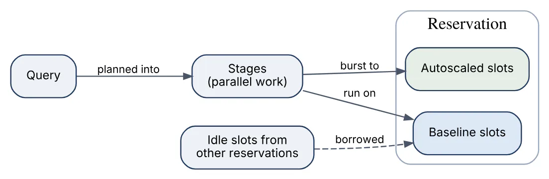
The Snowflake parallel is a multi-cluster warehouse with min and max cluster counts, except that BigQuery autoscaling is in slot increments across all queries rather than per whole cluster.
34In a real project using Snowflake / BigQuery, how would you apply, test, or troubleshoot BigQuery slots and reservations?
Apply. For a bank’s reporting platform I created one admin project with three reservations: etl (Enterprise, baseline 200, max 800, assigned to pipeline projects with job type PIPELINE), bi (baseline 100, max 400, assigned to the Looker project) and adhoc (baseline 0, max 200). Idle slot sharing is left on so the overnight ETL can borrow BI capacity. A one-year commitment covers the sum of the baselines because they run continuously anyway.
Test. Before go-live I replayed a week of production jobs from INFORMATION_SCHEMA.JOBS into the new reservations and checked that p95 job duration matched or beat on-demand. Capacity tests use the Slot Estimator in the console and the JOBS_TIMELINE_BY_ORGANIZATION view to see whether the max was hit; if period_slot_ms sits at the ceiling for more than ten minutes a day, the ceiling is too low. Cost is verified from the billing export grouped by reservation label.
Troubleshoot. Users in the BI project complain of queueing at 9 a.m. The timeline shows the reservation pinned at 400 slots while etl has 300 idle, yet sharing did not help because the ETL reservation was created with ignore_idle_slots = true for “predictability”. Turning it off solved the queueing. Another case: queries landed in on-demand despite the reservation because the assignment was made at project level but a Dataform job ran under a different project; INFORMATION_SCHEMA.JOBS.reservation_id revealed it.
Autoscaling adds slots in 50-slot increments billed for at least one minute, so many tiny spikes can cost more than a slightly higher baseline.
35Explain partitioning and clustering in BigQuery in the context of Snowflake / BigQuery.
Partitioning divides a BigQuery table into physical segments by one column: a DATE, TIMESTAMP or DATETIME column (daily, hourly, monthly or yearly), an integer range, or ingestion time (_PARTITIONTIME). A query that filters on the partition column scans only matching partitions, which directly reduces bytes billed on on-demand pricing. Tables are limited to 10,000 partitions, and require_partition_filter can make unfiltered queries fail outright.
Clustering sorts data within each partition (or the whole table if unpartitioned) by up to four columns. BigQuery keeps block-level min/max metadata so filters and aggregations on clustered columns skip blocks, and re-clusters automatically at no charge as data arrives. Clustered-column filters reduce bytes scanned too, but the estimate shown before running is an upper bound, since block pruning happens at execution.
CREATE TABLE sales.orders (
  order_id STRING, customer_id STRING, region STRING,
  amount NUMERIC, order_ts TIMESTAMP)
PARTITION BY DATE(order_ts)
CLUSTER BY region, customer_id
OPTIONS (require_partition_filter = TRUE,
         partition_expiration_days = 730);
Guidance: partition on the column that bounds almost every query (time), cluster on the next most selective filters or join keys, coarse before fine. Snowflake has no explicit partitions; its automatic micro-partitions plus an optional clustering key cover both roles.
36In a real project using Snowflake / BigQuery, how would you apply, test, or troubleshoot partitioning and clustering in BigQuery?
Apply. For a 40 TB ad-impressions table queried by date and advertiser, I partition by DATE(impression_ts) with require_partition_filter = TRUE and cluster by advertiser_id, campaign_id. Partitions older than 13 months expire automatically, satisfying the retention policy without a cleanup job. The staging table that receives streaming inserts is ingestion-time partitioned so the daily MERGE can target a single partition with WHERE _PARTITIONDATE = @day.
Test. Every new query in the repository passes a dry run; the CI job asserts totalBytesProcessed is below a per-query budget, which immediately catches a missing partition filter. For clustering effectiveness I compare total_bytes_billed in INFORMATION_SCHEMA.JOBS against the dry-run estimate: a large gap proves block pruning worked. Partition pruning is confirmed in the execution details, where the input stage shows the number of partitions read.
bq query --dry_run --use_legacy_sql=false \
  'SELECT advertiser_id, SUM(cost) FROM ads.impressions
   WHERE DATE(impression_ts) BETWEEN "2026-10-01" AND "2026-10-07"
   GROUP BY 1'
Troubleshoot. A dashboard query scans the full table despite a date filter. The filter was WHERE TIMESTAMP_TRUNC(impression_ts, DAY) = ... inside a subquery joined to another table, which BigQuery could not prune; rewriting with a literal range on DATE(impression_ts) in the outer WHERE restored pruning. Another incident: a MERGE touching all partitions daily caused the table to become fully clustered only after each run, so queries just after loading were slow until background reclustering finished.
Partition filters only prune when the predicate is a constant or parameter; comparing the partition column to another table’s column scans everything.
37Explain BigQuery nested repeated fields in the context of Snowflake / BigQuery.
BigQuery’s schema supports two composite types: STRUCT (a nested record with named fields) and ARRAY (a repeated field holding zero or more values of one type, including structs). Together they let a single row hold, for example, an order with an array of line items, each a struct of sku, qty and price. The data stays columnar inside Capacitor, so reading items.sku reads only that leaf, not the whole array.
Why it matters: denormalising one-to-many relationships into repeated fields avoids a join at query time and keeps parent and children co-located, which is the idiomatic BigQuery design for event and transaction data. Querying uses UNNEST to flatten an array into rows, typically with a correlated cross join.
SELECT o.order_id, i.sku, i.qty * i.price AS line_total
FROM   sales.orders AS o,
       UNNEST(o.items) AS i
WHERE  DATE(o.order_ts) = '2026-10-01';

-- aggregate without flattening the whole table
SELECT order_id,
       (SELECT SUM(qty) FROM UNNEST(items)) AS total_qty
FROM   sales.orders;
ARRAY_AGG(STRUCT(...)) rebuilds nested rows after a join. Snowflake covers the same ground with typed ARRAY and OBJECT, or VARIANT, flattened with LATERAL FLATTEN, but BigQuery’s version is strongly typed at the schema level, so column statistics and pruning apply to nested leaves.
38In a real project using Snowflake / BigQuery, how would you apply, test, or troubleshoot BigQuery nested repeated fields?
Apply. For a mobile analytics pipeline, each session row holds events ARRAY<STRUCT<name STRING, ts TIMESTAMP, params ARRAY<STRUCT<key STRING, value STRING>>>>, the same shape Firebase exports. Session-level questions read the top-level columns cheaply; funnel analysis unnests events only for the sessions in the date window. Product dimension tables stay flat, because a repeated field is right for parent-child data that is always queried together and wrong for shared reference data.
Test. Schema contracts are tested with bq show --schema diffed against the repository’s JSON schema in CI, since adding a nested field is backward compatible but changing a type is not. Data tests assert that ARRAY_LENGTH(events) > 0 for every session and that unnesting and re-aggregating with ARRAY_AGG returns the same row count, which catches accidental fan-out. For performance I compare bytes processed with and without the nested design on a representative query set.
Troubleshoot. A revenue report doubled overnight. The query cross-joined two UNNESTs (events and purchases) in the same FROM, multiplying rows; moving the second array into a correlated subquery fixed it. Another ticket: “query returns no rows for sessions without events”, because a comma UNNEST is an inner join; LEFT JOIN UNNEST(events) AS e keeps the parent. Lastly, a SELECT * on the nested table was costing far more than expected because it read every leaf column; selecting specific leaves cut bytes by 80%.
The trade-off is update cost: changing one line item means rewriting the whole parent row, so highly mutable child data fits a separate table better.
39Explain BigQuery materialized views in the context of Snowflake / BigQuery.
A BigQuery materialized view precomputes and stores the result of a query over one or more base tables and keeps it current automatically. BigQuery refreshes it incrementally in the background as base data changes, and, crucially, the optimizer rewrites queries against the base tables to use the view when it can (smart tuning), so users do not need to know the view exists. Reading from a materialized view is billed on the bytes it scans, which is normally far less than the base table.
CREATE MATERIALIZED VIEW sales.mv_daily_region_revenue
PARTITION BY order_day
CLUSTER BY region
OPTIONS (enable_refresh = TRUE, refresh_interval_minutes = 30,
         max_staleness = INTERVAL 1 HOUR)
AS
SELECT DATE(order_ts) AS order_day, region,
       SUM(amount) AS revenue, COUNT(*) AS orders
FROM   sales.orders
GROUP  BY 1, 2;
Constraints to know: aggregations must be incrementally maintainable (SUM, COUNT, MIN, MAX, APPROX_COUNT_DISTINCT), inner joins are supported, and allow_non_incremental_definition = TRUE relaxes the SQL restrictions in exchange for full refreshes. max_staleness lets a query read the possibly stale view without merging fresh base deltas, trading freshness for cost. Materialized views cannot be partitioned differently from their base table.
Snowflake materialized views are more restricted (single table, no joins, Enterprise edition), which is why dynamic tables are often the practical Snowflake equivalent.
40In a real project using Snowflake / BigQuery, how would you apply, test, or troubleshoot BigQuery materialized views?
Apply. A SaaS usage dashboard ran SUM and COUNT aggregates over a 20 TB events table every time someone opened it. I created a materialized view aggregating by day, tenant and feature with max_staleness = INTERVAL 30 MINUTE, partitioned on the day column. Nothing in Looker changed: smart tuning rewrote the dashboard queries to hit the view, and bytes processed per dashboard load fell from 2 TB to under 10 GB.
Test. Correctness is verified by running the view definition as a plain query and diffing against SELECT * FROM mv with max_staleness set to zero. To prove the rewrite is happening I check the job’s materialized_view_statistics in INFORMATION_SCHEMA.JOBS, which lists whether each candidate view was chosen or rejected and why. Refresh cost is monitored through INFORMATION_SCHEMA.JOBS where job_type = 'QUERY' and the statement type is a materialized view refresh, attributed to the reservation.
Troubleshoot. The dashboard went back to scanning the base table. materialized_view_statistics reported rejected_reason = BASE_TABLE_DATA_CHANGE: the view had not refreshed because a bulk backfill updated 18 months of history, invalidating most of it, and the refresh job was waiting for slots. Running a manual CALL BQ.REFRESH_MATERIALIZED_VIEW(...) from a reservation with free capacity restored acceleration. A second issue was a view that refused to be created because the query used COUNT(DISTINCT); APPROX_COUNT_DISTINCT or allow_non_incremental_definition were the options.
Remember that DML on the base table that touches many partitions turns incremental refresh into a near-full recompute, so materialized views suit append-heavy tables best.
41Explain BigQuery streaming ingestion in the context of Snowflake / BigQuery.
Streaming ingestion writes individual rows or small batches into a BigQuery table with second-level latency, as opposed to batch load jobs that import files for free. The current mechanism is the Storage Write API, a gRPC-based service with two main modes: the default stream for at-least-once, low-latency appends, and application-created streams (pending or committed types) that give exactly-once semantics through stream offsets and atomic commits. The older tabledata.insertAll (legacy streaming API) still works but costs more and offers only best-effort deduplication via insertId.
Rows arrive first in a streaming buffer and become queryable within seconds, then are flushed to managed storage. While rows sit in the buffer they cannot be modified by DML and UPDATE / DELETE on recent partitions may fail with “would affect rows in the streaming buffer” (a window of up to 90 minutes with the legacy API; the Write API commits directly).
Common producers are Dataflow (BigQueryIO with STORAGE_WRITE_API), Pub/Sub BigQuery subscriptions that write directly without any pipeline, Kafka Connect and the client libraries. Pricing is per GiB ingested, with a monthly free tier.
Snowflake’s equivalents are Snowpipe Streaming for row-level writes from an SDK or Kafka connector and classic Snowpipe for micro-batched files.
42In a real project using Snowflake / BigQuery, how would you apply, test, or troubleshoot BigQuery streaming ingestion?
Apply. For a payments platform emitting transaction events to Pub/Sub, I used a BigQuery subscription writing straight to an ingestion-time partitioned raw.transactions table with use_topic_schema, so no Dataflow job is needed for the simple case. Enrichment that requires lookups runs as a Dataflow pipeline using the Storage Write API in exactly-once mode, writing to curated.transactions. Both tables cluster by merchant_id so downstream merges and fraud queries prune.
Test. Latency and completeness are tested end to end: a load generator publishes 10,000 messages with sequential IDs, and a test query waits until COUNT(DISTINCT id) = 10000, measuring the p99 arrival delay. Duplicate tests restart the Dataflow job mid-stream and verify COUNT(*) = COUNT(DISTINCT id) in the exactly-once table while documenting the duplicates expected in the at-least-once one. Schema evolution is tested by adding an optional field to the Pub/Sub schema and confirming writes continue.
Troubleshoot. Messages piling up in the Pub/Sub dead-letter topic point to schema mismatches; the subscription’s error detail shows the field type that failed. Exceeded rate limits errors from the Write API mean too many concurrent streams or too-small append batches, fixed by batching rows and reusing a stream per worker. A downstream MERGE failing with the streaming-buffer error is handled by targeting partitions older than the buffer window or by moving the writer to the Storage Write API.
Streaming costs several times more per GiB than batch loads, so events that can wait a few minutes should be micro-batched through load jobs instead.
43Explain BigQuery storage and billing in the context of Snowflake / BigQuery.
BigQuery bills storage and compute separately. Storage is charged per GiB per month in one of two models chosen per dataset: logical (uncompressed size of the data, the default) or physical (compressed bytes actually stored, including time travel and fail-safe bytes, at a higher unit price). Physical billing usually wins for well-compressing data but loses on tables with heavy churn, so the decision is made per dataset after inspecting INFORMATION_SCHEMA.TABLE_STORAGE. Either way, data untouched for 90 consecutive days drops to the long-term rate, roughly half price, automatically.
Compute follows two pricing models:
| Model | Unit | Free tier | Controls |
|---|---|---|---|
| On-demand | Per TiB of bytes scanned | 1 TiB per month | maximum_bytes_billed, custom quotas |
| Editions | Per slot-hour (Standard, Enterprise, Enterprise Plus) | None | Baseline, autoscale max, commitments |
Other meters: streaming ingestion per GiB (batch loads are free), BI Engine per GiB-hour, Storage Read API per TiB read by external engines, and cross-region or internet egress. Queries that fail or hit cache are not billed on on-demand. The billing export to BigQuery itself, joined with INFORMATION_SCHEMA.JOBS, is the standard way to attribute cost to users and labels.
Snowflake’s model is per-second compute credits plus per-TB compressed storage; the clearest contrast is that Snowflake never bills by bytes scanned while BigQuery on-demand bills nothing else.
44In a real project using Snowflake / BigQuery, how would you apply, test, or troubleshoot BigQuery storage and billing?
Apply. On a 300 TB warehouse I run a monthly storage review: a query over INFORMATION_SCHEMA.TABLE_STORAGE_BY_PROJECT compares total_logical_bytes with total_physical_bytes per dataset, and datasets with compression ratios above about 2.5:1 and modest time_travel_physical_bytes are switched to physical billing. Raw landing datasets get a 7-day table expiration; large fact tables get partition expiration. Every job carries labels (team, pipeline), and the billing export feeds a Looker Studio chargeback report.
Test. Pricing changes are tested with arithmetic before being applied: the storage view gives the bytes, and I compute both models’ monthly cost in SQL to confirm the saving. For compute, every pipeline query has a dry-run assertion in CI, and the per-user custom quota (QueryUsagePerUserPerDay) is set in a sandbox project and verified by deliberately exceeding it.
SELECT table_schema,
       ROUND(SUM(total_logical_bytes) / POW(1024, 4), 2)  AS logical_tib,
       ROUND(SUM(total_physical_bytes) / POW(1024, 4), 2) AS physical_tib
FROM   `region-us`.INFORMATION_SCHEMA.TABLE_STORAGE_BY_PROJECT
GROUP  BY 1 ORDER BY 2 DESC;
Troubleshoot. A bill tripled in one week. INFORMATION_SCHEMA.JOBS_BY_PROJECT ordered by total_bytes_billed showed a new Looker explore running SELECT * on an unpartitioned 30 TB table every five minutes via a scheduled refresh; adding a partition filter and caching the explore fixed it. On the storage side, a dataset on physical billing suddenly cost more because a daily full-table CREATE OR REPLACE kept seven days of time travel bytes; shortening the time travel window to two days cut that.
The main caveat is that switching a dataset’s billing model is locked for 14 days after a change, so test the arithmetic rather than flip-flopping.
45Explain BigQuery SQL window functions in the context of Snowflake / BigQuery.
Window (analytic) functions compute a value for each row using a set of related rows defined by an OVER clause, without collapsing the rows the way GROUP BY does. The OVER clause has three optional parts: PARTITION BY to split rows into groups, ORDER BY to define sequence within the group, and a frame (ROWS BETWEEN ... or RANGE BETWEEN ...) to bound which rows the function sees.
Function families in BigQuery:
- Numbering —
ROW_NUMBER,RANK,DENSE_RANK,NTILE,PERCENT_RANK. - Navigation —
LAG,LEAD,FIRST_VALUE,LAST_VALUE,NTH_VALUE. - Aggregate as window —
SUM,AVG,COUNT,MIN,MAX,ARRAY_AGGwithOVER.
SELECT customer_id, order_ts, amount,
       SUM(amount) OVER (PARTITION BY customer_id ORDER BY order_ts
                         ROWS BETWEEN UNBOUNDED PRECEDING AND CURRENT ROW)
         AS running_total,
       LAG(order_ts) OVER (PARTITION BY customer_id ORDER BY order_ts)
         AS previous_order_ts
FROM sales.orders
QUALIFY ROW_NUMBER() OVER (PARTITION BY customer_id ORDER BY order_ts DESC) <= 3;
QUALIFY filters on window results without a subquery, and a named WINDOW clause lets several functions share one specification. Default frames matter: with ORDER BY and no frame, the default is RANGE UNBOUNDED PRECEDING TO CURRENT ROW, which includes peer rows with equal order values and surprises people computing running totals over duplicate timestamps. Snowflake’s window function syntax is almost identical, including QUALIFY.
46In a real project using Snowflake / BigQuery, how would you apply, test, or troubleshoot BigQuery SQL window functions?
Apply. In a subscription analytics model the three heaviest uses are deduplication of CDC records (ROW_NUMBER over the key ordered by updated_at DESC, filtered with QUALIFY ... = 1), sessionisation of events (LAG(ts) to compute gaps, then a running SUM of a new-session flag to assign session IDs), and retention cohorts (FIRST_VALUE(order_month) per customer). Each lives in its own dbt model so the window partitions line up with the table’s clustering columns.
Test. Window logic is tested with fixed fixtures: a seed table of ten customers with crafted edge cases (ties on timestamps, single-row partitions, NULL order values) and an expected-output table, compared with EXCEPT DISTINCT in both directions. For the dedup model a test asserts COUNT(*) = COUNT(DISTINCT key) on the output. Performance tests watch the execution details for a stage with heavy “repartition” time, which signals the shuffle caused by PARTITION BY.
Troubleshoot. A running total showed identical values for several rows per customer: the frame defaulted to RANGE, and duplicate order_ts values were treated as peers. Switching to ROWS BETWEEN UNBOUNDED PRECEDING AND CURRENT ROW fixed it. A query failing with Resources exceeded had ROW_NUMBER() OVER (ORDER BY ts) without PARTITION BY, forcing one worker to sort the whole table; adding a sensible partition or pre-filtering removed the global sort. LAST_VALUE returning the current row instead of the partition’s last row is the same default-frame trap.
The important point is that window functions never reduce rows, so filtering by their result requires QUALIFY or an outer query; WHERE cannot reference them.
47Explain BigQuery IAM and row-level security in the context of Snowflake / BigQuery.
BigQuery authorisation has two layers. Cloud IAM controls who can do what at project, dataset, table, view or routine level through roles bound to principals (users, groups, service accounts). Predefined roles include roles/bigquery.dataViewer, dataEditor, jobUser (run queries, billed to that project) and admin; dataset-level grants also accept READER / WRITER / OWNER legacy bindings. Access must combine data permission (view the table) with job permission (run a query in some project).
Finer control inside a table:
- Row-level security — a
ROW ACCESS POLICYattaches a filter predicate to a table for specified principals; rows not matching are invisible to them, including through views andCOUNT(*). - Column-level security — policy tags from Data Catalog on sensitive columns; only principals with the Fine-Grained Reader role on the tag can select them, and dynamic data masking can return hashed or null values instead.
- Authorized views / datasets — a view in one dataset is granted access to tables in another so consumers see only the view.
CREATE ROW ACCESS POLICY region_filter
ON sales.orders
GRANT TO ('group:emea-analysts@example.com')
FILTER USING (region = 'EMEA');
Once any policy exists on a table, principals without a matching policy see zero rows. Snowflake’s equivalents are row access policies and masking policies, also attached to tables and columns, but evaluated against roles rather than IAM principals.
48In a real project using Snowflake / BigQuery, how would you apply, test, or troubleshoot BigQuery IAM and row-level security?
Apply. For a multi-country retailer sharing one sales dataset, I grant dataViewer to a Google group per country and attach one row access policy per group filtering on country_code; a global analytics group gets a TRUE filter policy. Service accounts for pipelines hold dataEditor on the curated dataset and jobUser on their own project, never project-level admin. Policy tags mark PII columns, with masking returning SHA-256 hashes for analysts and raw values for the fraud team. Everything is declared in Terraform so a grant is a reviewed pull request.
Test. A CI job impersonates a test service account per group (--impersonate-service-account) and runs SELECT country_code, COUNT(*) ... GROUP BY 1, asserting only the expected country appears, and that SELECT email fails with a policy-tag permission error for the analyst identity. A policy inventory test queries INFORMATION_SCHEMA.TABLES and fails if any table containing PII tags lacks a row access policy when it should have one. Audit logs (data_access) are checked for the test identities to confirm reads were logged.
Troubleshoot. “I can see the table but get zero rows” means the user is not covered by any row access policy on that table; SHOW has no equivalent, so I list policies with the bq CLI or the ROW_ACCESS_POLICIES information schema view. “Permission denied on job” with correct data access means the user lacks jobUser in the billing project. A materialized view or BI Engine refusing to accelerate a table is often because row-level security is present, which disables those optimisations.
Row access policies are evaluated per query and add filter cost; they also block table copy, export and snapshot for restricted principals.
49Explain BigQuery external tables in the context of Snowflake / BigQuery.
An external table is a BigQuery table whose data stays outside BigQuery storage: Parquet, ORC, Avro, CSV or JSON files in Cloud Storage, data in Bigtable or Google Drive, or, through BigQuery Omni, files in Amazon S3 and Azure Blob Storage. BigQuery stores only the schema and location; each query reads the source directly, so there is no load step and no storage charge, but also no managed-storage features such as clustering, DML or time travel. BigLake tables are the governed form: access goes through a connection resource so users need no permission on the bucket, and they unlock fine-grained security, metadata caching and better performance.
CREATE EXTERNAL TABLE lake.raw_events
WITH PARTITION COLUMNS (event_date DATE)
WITH CONNECTION `us.gcs_lake_conn`
OPTIONS (
  format = 'PARQUET',
  uris = ['gs://acme-lake/events/*'],
  hive_partition_uri_prefix = 'gs://acme-lake/events',
  max_staleness = INTERVAL 4 HOUR,
  metadata_cache_mode = 'AUTOMATIC');
Hive-style partition folders (event_date=2026-10-01/) become pruning columns. On-demand billing counts bytes read from the files, so Parquet with partition filters is far cheaper than CSV. Typical uses are querying a data lake in place, one-time exploration before loading, and federating with Spanner or Cloud SQL via EXTERNAL_QUERY.
Snowflake external tables over S3, Azure or GCS stages, and Iceberg tables with external catalogs, are the equivalents.
50In a real project using Snowflake / BigQuery, how would you apply, test, or troubleshoot BigQuery external tables?
Apply. A manufacturing client lands sensor data as Parquet in a Cloud Storage lake owned by the platform team. Rather than duplicate 80 TB into BigQuery, I define BigLake tables with hive partitioning on plant_id and reading_date, metadata caching set to automatic, and a max_staleness of one hour so planners can tolerate slightly delayed file listings. Only the hot last 90 days are copied into a native clustered table for the sub-second dashboards; everything older is queried in place.
Test. Schema drift is the main risk, so a nightly job runs SELECT * FROM lake.sensor_readings LIMIT 0 and compares the inferred schema to the contract; a new Parquet file with a widened type fails the job before analysts hit errors. Partition pruning is verified by comparing total_bytes_processed for a filtered and an unfiltered query. For BigLake, a test identity without bucket permissions must still succeed through the connection, proving governance works.
Troubleshoot. Queries slowed down from seconds to minutes: thousands of 50 KB files had been written by a misconfigured Spark job, and listing them dominated runtime. Compacting to 256 MB to 1 GB files and enabling metadata caching fixed it. A Cannot read ... Parquet column type mismatch error came from one producer switching a column from INT64 to STRING; the fix was quarantining that day’s folder and reprocessing. “Access Denied” on a connection usually means the connection’s service account lacks storage.objectViewer on the bucket.
External data is only as fast as the file layout, and it cannot be clustered, snapshotted or benefit from long-term storage pricing.
51Explain BigQuery BI Engine in the context of Snowflake / BigQuery.
BI Engine is an in-memory analysis service that accelerates BigQuery queries by caching table data in RAM and executing supported query shapes with a vectorised engine. You reserve capacity per project and location, from 1 GiB up to 250 GiB by default (quota increases are possible), and pay per GiB-hour. Any client that issues SQL to BigQuery benefits automatically: Looker Studio, Looker, Tableau, Power BI or the API; there is no special connector any more.
How it behaves:
- BigQuery decides per query whether BI Engine can fully or partially accelerate it;
biEngineStatisticsin the job metadata reportsFULL,PARTIALorDISABLEDwith reason codes. - Preferred tables (
ALTER BI_CAPACITY ... SET OPTIONS (preferred_tables = [...])) restrict acceleration to specific tables so the reservation is not diluted. - Accelerated queries still produce normal job records but process bytes from memory; on-demand pricing is still charged per bytes scanned, while reservations consume no slots for the accelerated part.
- Unsupported constructs (some window functions, UDFs, external tables, row-level security) fall back to normal execution.
It fits dashboards with many small, repetitive aggregate queries over a bounded dataset. Snowflake has no in-memory BI tier; its equivalents are the result cache, warehouse local SSD cache and keeping a BI warehouse warm.
52In a real project using Snowflake / BigQuery, how would you apply, test, or troubleshoot BigQuery BI Engine?
Apply. An executive Looker Studio dashboard over a 30 GB pre-aggregated kpi_daily table served 400 users and regularly took five to eight seconds per tile. I reserved 32 GiB of BI Engine in the dashboard project and set preferred_tables to the three KPI tables so ad hoc queries elsewhere would not evict them. Tiles dropped to well under a second, and because the project uses an Enterprise reservation, accelerated tiles stopped consuming slots during the 9 a.m. peak.
Test. Acceptance was measured, not assumed: a Locust script replayed the dashboard’s query log for one hour before and after the reservation and compared p50/p95 latencies. For each query I checked bi_engine_statistics.bi_engine_mode in INFORMATION_SCHEMA.JOBS; anything DISABLED was reviewed for its reason code. Memory sizing was validated with the reservation/used_bytes monitoring metric, aiming for under 80% utilisation.
SELECT bi_engine_statistics.bi_engine_mode AS mode, COUNT(*) AS jobs,
       ROUND(AVG(TIMESTAMP_DIFF(end_time, start_time, MILLISECOND))) AS avg_ms
FROM   `region-us`.INFORMATION_SCHEMA.JOBS_BY_PROJECT
WHERE  creation_time > TIMESTAMP_SUB(CURRENT_TIMESTAMP(), INTERVAL 1 DAY)
GROUP  BY 1;
Troubleshoot. Acceleration silently stopped after a release. The reason code was UNSUPPORTED_SQL_TEXT: a new tile used a PERCENTILE_CONT window function. Replacing it with a pre-computed column restored full acceleration. Another dashboard reported INSUFFICIENT_RESERVATION: the underlying table had grown past the reserved memory; the fix was a smaller aggregate table rather than more GiB. Tables with row-level security were never accelerated, which explained one team’s “it never worked for us”.
BI Engine is a per-project, per-location resource, so a dashboard pointing at tables in another region gains nothing.
53Explain BigQuery scheduled queries in the context of Snowflake / BigQuery.
A scheduled query is a saved SQL statement that BigQuery runs on a recurrence (hourly, daily, custom cron) under the Data Transfer Service, writing results to a destination table or executing DDL/DML such as MERGE. It is the lightest way to orchestrate transformations without Airflow or Dataform. Configuration includes the schedule, destination, write disposition (WRITE_TRUNCATE, WRITE_APPEND) or partition decorator, the service account to run as, notification options (email, Pub/Sub topic) and an optional start and end time.
Parameters make backfills clean: @run_time and @run_date are available inside the query, and the destination can be events_summary${run_date} to write exactly one partition per run. Historical runs can be scheduled for a date range and execute in parallel.
MERGE curated.daily_sales AS t
USING (
  SELECT DATE(order_ts) AS day, region, SUM(amount) AS revenue
  FROM   raw.orders
  WHERE  DATE(order_ts) = DATE_SUB(@run_date, INTERVAL 1 DAY)
  GROUP  BY 1, 2) AS s
ON t.day = s.day AND t.region = s.region
WHEN MATCHED THEN UPDATE SET revenue = s.revenue
WHEN NOT MATCHED THEN INSERT ROW;
Run history and errors live in the transfer configuration and in INFORMATION_SCHEMA.JOBS (jobs are labelled with the transfer config). Limits: no dependencies between queries and no retries beyond the service’s own, so chains belong in Dataform, Cloud Composer or Workflows. Snowflake’s equivalent is a task with a SCHEDULE, which additionally supports DAG dependencies via AFTER.
54In a real project using Snowflake / BigQuery, how would you apply, test, or troubleshoot BigQuery scheduled queries?
Apply. A marketing team needed a daily campaign-performance table but no engineering orchestration existed. I built the transformation as a scheduled query running at 05:30 under a dedicated service account with dataEditor on the target dataset only, writing to campaign_daily$ {run_date} with WRITE_TRUNCATE so each run is idempotent per partition. Failure notifications go to a Pub/Sub topic that a Cloud Function forwards to Slack. When the team’s needs grew to six dependent steps, I migrated the SQL unchanged into Dataform.
Test. The query is first run manually with @run_date bound to a known date and the output compared to a hand-computed expectation. A backfill of a 30-day range verifies idempotency: running the same date twice yields identical partition contents and no duplicate rows. In CI, the SQL file is dry-run against production schemas so a renamed source column fails the build, not the 05:30 run.
Troubleshoot. “The table is stale” with no error usually means the schedule ran but the source had not yet loaded, a race rather than a failure; adding a guard (ASSERT (SELECT COUNT(*) FROM raw.orders WHERE DATE(order_ts) = ...) > 0) makes the run fail loudly, and shifting the schedule or moving to event-driven orchestration solves it properly. A run failing with Access Denied after months of success typically follows a change of the owning user’s permissions; moving the configuration to a service account removes the human dependency. Partition-decorator writes that suddenly create a table named campaign_daily$20261001 literally mean the destination table lost its partitioning.
Scheduled queries are convenient but opaque; once there are dependencies, retries or more than a handful of them, a proper orchestrator pays for itself.
55Explain BigQuery performance optimization in the context of Snowflake / BigQuery.
Performance in BigQuery is mostly about reducing bytes read, reducing shuffle, and giving the engine enough slots. The levers in rough order of impact:
- Scan less — select only needed columns (columnar storage makes
SELECT *the worst habit), filter on the partition column with constants, cluster on common filters and join keys. - Pre-aggregate — materialized views, summary tables from scheduled queries, or BI Engine for repeated dashboard shapes.
- Shape joins well — put the larger table first, filter before joining, avoid joins on computed expressions, and break up skewed keys (a handful of
customer_idvalues with millions of rows each stall one slot). - Avoid global sorts —
ORDER BYwithoutLIMITon huge results andROW_NUMBERwithoutPARTITION BYserialise onto one worker. - Use approximate functions —
APPROX_COUNT_DISTINCT,APPROX_QUANTILESwhen exactness is not required. - Mind semi-structured data —
JSONcolumns are parsed at read time; promote hot keys to real columns. - Give it capacity — a reservation with headroom removes the on-demand slot ceiling.
Diagnosis uses the query plan’s execution details: per-stage wait, read, compute and write ratios, records in and out, and the “slot contention” and “shuffle spilled to disk” indicators. INFORMATION_SCHEMA.JOBS adds total_slot_ms, total_bytes_billed and query_info.performance_insights, which names stage-level problems such as high input skew. Snowflake’s Query Profile and pruning statistics serve the same purpose with warehouse size as the extra dial.
56In a real project using Snowflake / BigQuery, how would you apply, test, or troubleshoot BigQuery performance optimization?
Apply. For a logistics warehouse whose daily dbt run grew from 40 minutes to over three hours, I attacked the five slowest models from INFORMATION_SCHEMA.JOBS. Two were fixed by adding partition filters to incremental models (WHERE DATE(event_ts) >= DATE_SUB(@run_date, INTERVAL 3 DAY)); one by clustering the shipment table on carrier_id, which the biggest join used; one by replacing COUNT(DISTINCT device_id) with APPROX_COUNT_DISTINCT in a monitoring table; and one by pre-aggregating a 2 TB fact into a daily summary that four downstream models now read.
Test. Each change is measured with the same inputs: I run before and after against a frozen snapshot table, record total_slot_ms and total_bytes_billed, and keep the change only if slot time drops meaningfully. CI enforces dry-run byte budgets per model, and a weekly report lists models whose slot time grew more than 30% week over week so regressions surface before users complain.
Troubleshoot. A query stuck at 95% for twenty minutes showed one stage with records-in massively skewed: a NULL join key matched millions of rows on both sides. Filtering NULL keys before the join finished the query in two minutes. Another slow query had performance_insights.stage_performance_standalone_insights.slot_contention = TRUE; the fix was capacity, not SQL, so it moved into the pipeline reservation. A dashboard query reading a 500 GB JSON column was rewritten to read three promoted columns, cutting bytes by 95%.
Most BigQuery performance problems are cost problems in disguise: fewer bytes and less shuffle make queries both faster and cheaper, so optimise the scan before adding slots.
57Explain BigQuery versus Snowflake trade-offs in the context of Snowflake / BigQuery.
Both are cloud-native, columnar, separated-storage-and-compute warehouses with ANSI SQL, semi-structured support, time travel, cloning and data sharing. The differences that drive a choice are operational model, cloud footprint and ecosystem.
| Dimension | BigQuery | Snowflake |
|---|---|---|
| Compute model | Serverless slots; no sizing | User-managed virtual warehouses |
| Pricing | Bytes scanned or slot-hours | Credits per second per warehouse |
| Cloud | Google Cloud only (Omni reads S3/Azure) | AWS, Azure, GCP; cross-cloud replication |
| Ecosystem | Tight GCP: Pub/Sub, Dataflow, Vertex AI, Looker | Marketplace, Snowpark, broad partner tooling |
| Isolation | Reservations and per-project quotas | Warehouse per workload, hard isolation |
Practical consequences: BigQuery removes capacity management and makes bursty, unpredictable analytics cheap to start, but cost control is about bytes and byte budgets. Snowflake makes workload isolation and cost attribution explicit through warehouses, which many enterprises find easier to govern, at the price of someone owning sizing decisions. BigQuery’s nested types and ML in SQL are more mature; Snowflake’s data sharing and multi-cloud story are stronger. Streaming is first class in both (Storage Write API, Snowpipe Streaming).
The honest answer in an interview is that organisations already on Google Cloud rarely regret BigQuery and multi-cloud or AWS-centric organisations rarely regret Snowflake; the SQL skills transfer almost entirely.
58In a real project using Snowflake / BigQuery, how would you apply, test, or troubleshoot BigQuery versus Snowflake trade-offs?
Apply. When a retailer with its applications on AWS and its marketing stack on Google Cloud asked which warehouse to adopt, I framed the decision around three facts rather than feature lists: 80% of source data was in S3 and Kinesis, the analytics team wanted strict per-department chargeback, and Google Ads and GA4 exports arrive natively in BigQuery. The recommendation was Snowflake on AWS as the enterprise warehouse with Snowflake’s GA4 connector and S3 ingestion, and a small BigQuery footprint left in place for the marketing team’s native exports, bridged through scheduled extracts to S3.
Test. A two-week proof of concept loaded the same 5 TB sample into both platforms and ran the same 30 representative queries plus a 100-user concurrency replay. Results were recorded for cost per query, p95 latency, time to onboard a new source and effort to implement row-level security. Both products passed on performance; the decision was made on cost predictability and ingestion fit, which is typical.
Troubleshoot. The failure mode of such decisions is surprise cost after migration. On the BigQuery side I have seen on-demand bills explode because analysts used to warehouse pricing wrote SELECT * freely; the fix was byte quotas and a reservation. On the Snowflake side, teams accustomed to serverless left warehouses running without auto-suspend; resource monitors fixed it. Cross-platform bridging fails when timezone and NUMERIC precision semantics differ, so reconciliation tests on row counts and sums per day caught several silent mismatches.
A trade-off decision should be revisited when the data gravity changes, not when a vendor announces a feature.
59Explain CDC data ingestion into Snowflake in the context of Snowflake / BigQuery.
Change data capture ingestion replicates inserts, updates and deletes from an operational database into Snowflake by reading the source’s transaction log rather than polling tables. A CDC tool (Debezium on Kafka, Fivetran, Qlik Replicate, AWS DMS, Oracle GoldenGate, or Snowflake’s own Openflow and database connectors) emits change events; those land in Snowflake through Snowpipe Streaming, the Kafka connector or file-based Snowpipe into an append-only change table; a stream and task or a dynamic table then applies the changes to a current-state table with MERGE.
The pipeline below is the common pattern.

Design points: keep the raw change log (it is the audit trail and enables SCD2), order events by the source LSN or commit timestamp rather than arrival time, handle deletes explicitly (op = 'd'), and apply only the latest change per key per batch with QUALIFY ROW_NUMBER() ... = 1 before merging. Schema evolution on the source must propagate; Snowpipe Streaming and the Kafka connector support schematization that adds columns automatically.
BigQuery’s parallel is Datastream writing to BigQuery with max_staleness CDC tables, or the Storage Write API’s _CHANGE_TYPE pseudo-column for upserts and deletes.
60In a real project using Snowflake / BigQuery, how would you apply, test, or troubleshoot CDC data ingestion into Snowflake?
Apply. For an order-management system on PostgreSQL I ran Debezium into Kafka and the Snowflake Kafka connector in Snowpipe Streaming mode into raw.orders_cdc, which keeps every change with op, source_lsn and ts_ms. A dynamic table with a five-minute target lag derives curated.orders_current by taking the latest change per order_id and dropping rows whose last op is a delete; a second dynamic table builds the SCD2 history. The initial load used a Debezium snapshot so the same code path handled both backfill and ongoing changes.
Test. Reconciliation is the core test: hourly, a query compares COUNT(*) and SUM(amount) per day in orders_current with the same figures pulled from a Postgres read replica, alerting on any difference. Chaos tests kill the connector mid-batch and confirm no duplicates (Snowpipe Streaming offsets are exactly-once per channel) and no gaps after restart. A schema test adds a nullable column in Postgres and checks it appears in Snowflake within one lag interval.
SELECT order_id, op, amount, status
FROM raw.orders_cdc
QUALIFY ROW_NUMBER() OVER (PARTITION BY order_id ORDER BY source_lsn DESC) = 1
  AND op <> 'd';
Troubleshoot. Reconciliation drifted by a few rows a day. The cause was ordering by ts_ms, where two updates within the same millisecond could land in the wrong order; switching to source_lsn fixed it. Replication lag spikes traced to the connector’s buffer flush settings and a Postgres replication slot that filled the WAL disk after a long connector outage, so slot monitoring became part of the runbook. A silent problem was Postgres TOAST columns omitted from update events, which Debezium marks with a placeholder; merging only non-placeholder columns solved it.
CDC gives you the source’s correctness, not business correctness: if the application soft-deletes, the warehouse must honour that flag rather than wait for a physical delete.
61Explain BigQuery table snapshots and time travel in the context of Snowflake / BigQuery.
BigQuery time travel lets you read a table as it was at any moment within the dataset’s time travel window, between two and seven days (default seven), using FOR SYSTEM_TIME AS OF. The same window supports restoring a deleted table (bq cp table@<epoch_ms> newtable or CREATE TABLE ... COPY ... FOR SYSTEM_TIME AS OF). After the window closes, a further seven-day fail-safe keeps the data recoverable only through Google support.
A table snapshot is a read-only, point-in-time copy that persists as long as you want (or until an expiration you set). It shares storage with the base table and is billed only for data that has since changed or been deleted in the base, which makes daily or weekly snapshots cheap for stable tables. Snapshots can be created from the current state or from any time within the time travel window, and restored into a writable table at any time.
CREATE SNAPSHOT TABLE sales.orders_snap_20261101
CLONE sales.orders FOR SYSTEM_TIME AS OF TIMESTAMP '2026-11-01 00:00:00 UTC'
OPTIONS (expiration_timestamp = TIMESTAMP '2027-02-01 00:00:00 UTC');

CREATE TABLE sales.orders_restored CLONE sales.orders_snap_20261101;
Table clones are the writable cousin, billed the same incremental way. Snowflake’s equivalents are Time Travel (1 to 90 days), Fail-safe, and zero-copy clones, which serve both the snapshot and clone roles.
62In a real project using Snowflake / BigQuery, how would you apply, test, or troubleshoot BigQuery table snapshots and time travel?
Apply. In a regulated finance warehouse I keep the time travel window at seven days on curated datasets for quick self-service recovery, but two days on high-churn staging datasets to reduce physical storage bills. A scheduled query creates a snapshot of every reporting table at month end with a 13-month expiration, giving auditors an immutable copy of exactly what was reported, and a snapshot is taken immediately before every schema migration so rollback is a CLONE.
Test. The recovery runbook is exercised quarterly: delete a test table, restore it via bq cp with a timestamp decorator, and compare a checksum (FARM_FINGERPRINT over sorted rows) with the pre-deletion value. Snapshot integrity tests confirm the snapshot’s row count equals the base table’s at the snapshot timestamp, computed with FOR SYSTEM_TIME AS OF. Storage cost tests query INFORMATION_SCHEMA.TABLE_STORAGE to confirm snapshot bytes stay close to the delta rather than the full table.
Troubleshoot. A restore returned “table not found at that timestamp”: the table had been dropped and recreated with the same name, which starts a new time travel history, and the snapshot of the old one existed only in the fail-safe period, requiring a support ticket. On the cost side, snapshots of a table rebuilt daily with CREATE OR REPLACE cost almost as much as full copies, because every byte differs after each rebuild; switching the pipeline to MERGE made them cheap again.
Snapshots are not cross-region backups: a regional outage takes them with the base table, so critical datasets also need cross-region replication or exports to Cloud Storage.
63Explain Snowflake data quality checks in the context of Snowflake / BigQuery.
Data quality checks verify that tables meet expectations about completeness, uniqueness, validity, freshness and consistency, and fail or alert when they do not. In Snowflake there are three common layers.
- Constraints and typing —
NOT NULLis enforced; primary and unique keys are declared but not enforced, so they document intent only. Strong column types andTRY_CASTat load catch malformed values early. - Data Metric Functions (DMFs) — Snowflake’s native framework (Enterprise edition and above). System DMFs such as
SNOWFLAKE.CORE.NULL_COUNT,DUPLICATE_COUNT,UNIQUE_COUNT,ROW_COUNT,FRESHNESSand custom DMFs are attached to tables withALTER TABLE ... ADD DATA METRIC FUNCTIONand run on aDATA_METRIC_SCHEDULE(minutes, cron or on DML). Results land inSNOWFLAKE.LOCAL.DATA_QUALITY_MONITORING_RESULTS, and alerts can be driven from that view. - Pipeline tests — dbt tests, Great Expectations or Soda run assertions as SQL after each load and block downstream models.
ALTER TABLE curated.orders SET DATA_METRIC_SCHEDULE = 'TRIGGER_ON_CHANGES';
ALTER TABLE curated.orders ADD DATA METRIC FUNCTION
  SNOWFLAKE.CORE.NULL_COUNT ON (customer_id);
ALTER TABLE curated.orders ADD DATA METRIC FUNCTION
  SNOWFLAKE.CORE.DUPLICATE_COUNT ON (order_id);
Freshness checks and row-count anomaly detection matter as much as nulls, because the most damaging failures are silent loads of nothing. BigQuery’s counterparts are the ASSERT statement inside pipelines, Dataform assertions and Dataplex auto data quality scans.
64In a real project using Snowflake / BigQuery, how would you apply, test, or troubleshoot Snowflake data quality checks?
Apply. For a claims warehouse the quality strategy had two tiers. Blocking checks run inside the dbt DAG: unique and not_null on every key, accepted_values on status codes, and a relationship test from claims to policies; a failure stops the publish step so dashboards keep yesterday’s good data. Observational checks use DMFs on the published tables: FRESHNESS on loaded_at, ROW_COUNT, and a custom DMF comparing total paid amount with the finance ledger; a Snowflake alert emails the data owner when a metric crosses a threshold.
Test. The checks themselves are tested by injecting known defects into a cloned schema: a duplicated claim, a null policy number, a stale load timestamp. Each injected defect must trip exactly the expected test, and the alert must fire within one scheduling interval. Thresholds are calibrated against 90 days of history in DATA_QUALITY_MONITORING_RESULTS so alerts are rare but meaningful.
Troubleshoot. A DUPLICATE_COUNT alert fired every morning at 03:10. The source was a backfill task that inserted before the dedup task ran; the metric was correct, the schedule was wrong, so the DMF schedule moved to TRIGGER_ON_CHANGES and the dedup moved into the same task DAG. Another case: FRESHNESS never alerted even though data was two days old, because the metric measured the DML timestamp of the table rather than the business timestamp; the fix was a custom DMF on MAX(event_date).
DMFs consume serverless credits per evaluation, so attach them to curated tables that people consume rather than to every raw landing table.
65Explain BigQuery ML in the context of Snowflake / BigQuery.
BigQuery ML lets you create, train, evaluate and run machine learning models with SQL, on data where it already lives, without moving it to a separate training environment. CREATE MODEL trains on the result of a SELECT; ML.EVALUATE, ML.PREDICT, ML.EXPLAIN_PREDICT and ML.FORECAST consume the model. Training is billed as query processing (on-demand bytes or slots) for built-in models, and feature preprocessing such as one-hot encoding and scaling happens automatically.
Supported model families include linear and logistic regression, k-means clustering, matrix factorisation for recommendations, boosted trees (XGBoost), deep neural networks, AutoML tables, ARIMA_PLUS time-series forecasting, principal component analysis and anomaly detection. Remote models connect to Vertex AI endpoints, including Gemini, so ML.GENERATE_TEXT and ML.GENERATE_EMBEDDING run LLM inference from SQL. Models can also be imported (TensorFlow, ONNX, XGBoost) or exported for serving elsewhere.
CREATE OR REPLACE MODEL churn.logreg_v1
OPTIONS (model_type = 'LOGISTIC_REG', input_label_cols = ['churned'],
         data_split_method = 'AUTO_SPLIT')
AS
SELECT tenure_months, monthly_spend, support_tickets, plan, churned
FROM   churn.training_set;

SELECT * FROM ML.EVALUATE(MODEL churn.logreg_v1);
SELECT customer_id, predicted_churned_probs
FROM   ML.PREDICT(MODEL churn.logreg_v1, TABLE churn.scoring_set);
Snowflake’s equivalent is Snowflake ML: the Snowpark ML Python library and the Model Registry, plus SQL ML functions for forecasting, anomaly detection and classification, and Cortex functions for LLM inference.
66In a real project using Snowflake / BigQuery, how would you apply, test, or troubleshoot BigQuery ML?
Apply. A telecom wanted a weekly churn score for 12 million subscribers without standing up a Vertex AI pipeline. Features are built in a dbt model (churn.features_weekly, partitioned by as_of_date), a scheduled query retrains a BOOSTED_TREE_CLASSIFIER monthly on the last 12 months, and another scheduled query writes ML.PREDICT output into churn.scores each Monday for the retention team’s dashboard. ML.EXPLAIN_PREDICT gives per-customer top features, which the agents actually read.
Test. Model quality gates run before any new model version is promoted: ML.EVALUATE on a held-out month must show ROC AUC above 0.80 and precision at the top decile above the current production model, otherwise the scheduled query keeps the old model. Data drift is monitored by comparing feature distributions (ML.FEATURE_INFO) between training and scoring sets. Scoring pipeline tests assert every active subscriber receives exactly one score per week.
Troubleshoot. Scores degraded over two months; ML.FEATURE_INFO showed the monthly_spend feature had switched currency units in the source, so the retrain job ingested shifted data. The fix was a quality check upstream and a retrain. A CREATE MODEL that ran for hours and failed with a resource error was training on a 1 TB table with data_split_method = 'RANDOM'; downsampling the majority class and clustering the training table cut it to minutes. Perfect AUC of 1.0 in evaluation turned out to be leakage: a cancellation_date feature was present for churned customers only.
BigQuery ML is excellent for tabular models that live near the data, but training cost scales with bytes processed, so retrain on what changed, not on history every time.
67Explain data warehouse schema design in the context of Snowflake / BigQuery.
Warehouse schema design decides how analytical data is organised for query performance, understandability and change tolerance. The dominant approach is dimensional modelling: fact tables hold measurable events at a declared grain (one row per order line), dimension tables hold descriptive context (customer, product, date), and facts reference dimensions through surrogate keys. A star schema keeps dimensions flat; a snowflake schema normalises them into sub-dimensions, which saves little in a columnar warehouse and adds joins. Data Vault (hubs, links, satellites) suits highly auditable, many-source integration layers, and One Big Table (OBT) denormalises everything for a specific consumer.
Cloud-specific adjustments:
- Columnar compression makes wide, denormalised tables cheap, so both platforms favour star schemas or OBT over heavily normalised designs.
- BigQuery adds nested and repeated fields, so order lines can live inside the order row instead of a separate fact.
- Snowflake’s
VARIANTlets you keep a raw layer loosely typed and model it later, the medallion (bronze/silver/gold) layering. - Partition and cluster facts by the time column and the most common filter; dimensions rarely need either.
- Slowly changing dimensions: type 1 overwrite, type 2 versioned rows with effective dates, implemented today with
MERGEor dbt snapshots.
Declared primary and foreign keys are informational in both platforms, so integrity is enforced by the pipeline, not the engine.
68In a real project using Snowflake / BigQuery, how would you apply, test, or troubleshoot data warehouse schema design?
Apply. For an e-commerce warehouse on Snowflake I used three layers: RAW (VARIANT landing tables, transient), CORE (a star schema with fct_order_line at the line grain, dim_customer as SCD2, dim_product, dim_date), and MART (wide, denormalised tables per business domain built from CORE). The grain of each fact is written in the model’s documentation and enforced by a uniqueness test on the grain columns. Surrogate keys are hashes of the natural key plus effective date so loads are deterministic and rerunnable.
Test. Schema quality is tested like code: uniqueness on the fact grain, referential tests that every fact key exists in its dimension (with a documented “unknown” member for late-arriving dimensions), and SCD2 tests that no customer has overlapping validity periods and exactly one current row. A performance test runs the top 20 BI queries and checks partitions scanned; if a mart requires joining five dimensions on every dashboard load, it is denormalised further.
Troubleshoot. Revenue in the mart exceeded finance by 4%: a fact at order-line grain had been joined to a shipment table at shipment grain, fanning out lines with multiple shipments. The fix was aggregating shipments to the line grain before joining and adding a row-count assertion. A second issue was dashboard slowness caused by a type 2 customer dimension with 200 million rows joined on a non-clustered key; adding a type 1 dim_customer_current for most reports solved it.
Grain is the decision that everything else depends on; changing it after consumers exist is the most expensive mistake in warehouse design.
69Explain ETL versus ELT in the context of Snowflake / BigQuery.
ETL extracts data from sources, transforms it on a separate processing engine (Informatica, SSIS, Spark clusters), then loads the finished result into the warehouse. ELT extracts, loads the raw data into the warehouse first, and transforms it there with SQL. Snowflake and BigQuery pushed the industry to ELT because their compute scales elastically, their SQL handles semi-structured data, and storing raw data is cheap.
| Aspect | ETL | ELT |
|---|---|---|
| Where transforms run | External engine before load | Inside the warehouse after load |
| Raw data retained | Usually not | Yes, enabling reprocessing and audit |
| Tooling | Informatica, Talend, Spark jobs | dbt, Dataform, tasks, dynamic tables, scheduled queries |
| Typical latency | Batch, longer pipelines | Near-real-time possible with streaming load |
| Fit | Heavy pre-load cleansing, legacy targets | Cloud warehouses with elastic compute |
ELT in practice: Fivetran or Snowpipe lands raw tables, dbt builds staging, core and mart layers as versioned SQL with tests, and the warehouse’s own engine does the work. ETL still earns its place when transformations need libraries SQL lacks, when PII must be masked before it ever reaches the warehouse, or when the source is a mainframe extract that needs heavy parsing. Many pipelines are hybrids: light transformation in flight (Dataflow, Snowpark), the rest in SQL.
The diagram shows an ELT pipeline where all transformation happens inside the warehouse.

Both platforms are equally suited to ELT; BigQuery’s Dataform and Snowflake’s dynamic tables are each vendor’s native answer to orchestrating the T.
70In a real project using Snowflake / BigQuery, how would you apply, test, or troubleshoot ETL versus ELT?
Apply. Migrating an insurer’s nightly Informatica ETL to BigQuery, I kept extraction as is (files to Cloud Storage), replaced the transformation tier with load-then-transform: load jobs land raw files into a raw dataset partitioned by load date, Dataform builds staging and reporting layers in SQL with assertions, and only one component stayed as pre-load processing: a Dataflow job that tokenises national ID numbers before anything is written to BigQuery, because compliance required that PII never land unmasked. Processing time dropped from six hours to forty minutes because the transformations ran on BigQuery slots instead of a four-node ETL server.
Test. The migration test was parallel running: for three weeks both pipelines produced the reporting tables, and a reconciliation query compared row counts and column-level checksums per table and day, with every mismatch triaged to a specific transformation rule. Dataform assertions covered uniqueness and referential rules that Informatica had enforced implicitly. Reprocessing was tested by deleting a day of staging data and rebuilding from raw, which the old ETL could not do at all.
Troubleshoot. Two post-migration incidents stand out. Costs rose because every Dataform model rebuilt entire tables nightly; converting the large facts to incremental models with partition filters fixed it. A subtler one was ordering semantics: Informatica had applied business rules in a specific sequence that the SQL version expressed as independent models, producing different results for records updated twice in a day; making the dependency explicit in the DAG restored parity.
ELT concentrates all compute cost in the warehouse, so without incremental models and byte budgets the saving in infrastructure can reappear on the query bill.
71Explain data governance lineage in the context of Snowflake / BigQuery.
Data governance is the set of policies and controls that decide who may use which data and how; lineage is the record of where data came from and what was derived from it. Lineage answers two questions: “which upstream sources and transformations produced this column?” and “what breaks or is exposed if I change or delete this one?”
Snowflake provides governance and lineage natively:
- Object tagging classifies objects and columns (
PII,CONFIDENTIAL), and tag-based masking policies apply protection automatically wherever a tag is set. - Classification detects likely personal data and suggests tags.
- Access History (
SNOWFLAKE.ACCOUNT_USAGE.ACCESS_HISTORY) records, per query, the base objects and columns read and written, including column-level source-to-target mapping for writes. Snowsight’s lineage graph is built from it (Enterprise edition and above). - Row access and masking policies enforce the rules.
BigQuery’s equivalent is Dataplex Universal Catalog: automatic lineage captured from BigQuery jobs (queries, loads, copies, scheduled queries) and from integrated tools such as Dataform, Dataflow and Composer, shown as a graph down to column level. Policy tags and business glossaries cover classification, and the Lineage API accepts events from tools it does not capture itself.
Lineage is observed from executed jobs, not declared, so it shows only what has actually run within the retention window (30 days in Dataplex) and cannot see transformations performed outside the platform.
72In a real project using Snowflake / BigQuery, how would you apply, test, or troubleshoot data governance lineage?
Apply. In a bank’s Snowflake estate, a classification job tags columns as PII_DIRECT, PII_INDIRECT or PUBLIC, and a single tag-based masking policy masks every PII_DIRECT column for non-privileged roles. When a regulator asks which reports contain customer national IDs, I walk ACCESS_HISTORY downstream from the tagged source columns instead of grepping SQL. Before every column deprecation, the pull-request check lists dependent objects from the same data.
Test. Controls are tested the way code is. A test role queries every table carrying PII_DIRECT and asserts the values come back masked. A lineage test runs a known INSERT ... SELECT in a sandbox and verifies ACCESS_HISTORY reports the expected source and target columns, so we know capture works before relying on it in an audit. A coverage query flags columns whose names match patterns such as ssn or email but carry no tag.
SELECT query_start_time, user_name,
       f.value:objectName::STRING AS source_table
FROM   snowflake.account_usage.access_history,
       LATERAL FLATTEN(base_objects_accessed) f
WHERE  f.value:objectName::STRING = 'CORE.CUSTOMER'
  AND  query_start_time > DATEADD(day, -7, CURRENT_TIMESTAMP());
Troubleshoot. A new dashboard exposed an unmasked email. Lineage showed a derived table created through CREATE TABLE AS SELECT before tagging existed, so it never inherited the tag; tag propagation applies only to objects created after the tag is attached. We re-tagged and added a nightly check. On BigQuery, a missing lineage edge usually means the job ran in a project or region where the Lineage API was not enabled.
Access History has up to a few hours of latency, so lineage is an audit tool, not a real-time guard.
73Explain warehouse concurrency performance in the context of Snowflake / BigQuery.
Concurrency performance is how well a warehouse keeps latency stable when many queries arrive at once. In Snowflake a virtual warehouse has a fixed amount of compute; when running queries exhaust it, new ones queue (MAX_CONCURRENCY_LEVEL, default 8, is a hint that governs how many run before queuing, and STATEMENT_QUEUED_TIMEOUT_IN_SECONDS bounds the wait). Queue time shows up as queued_overload_time in query history.
The diagram shows queries queuing when a cluster is saturated and a second cluster starting.
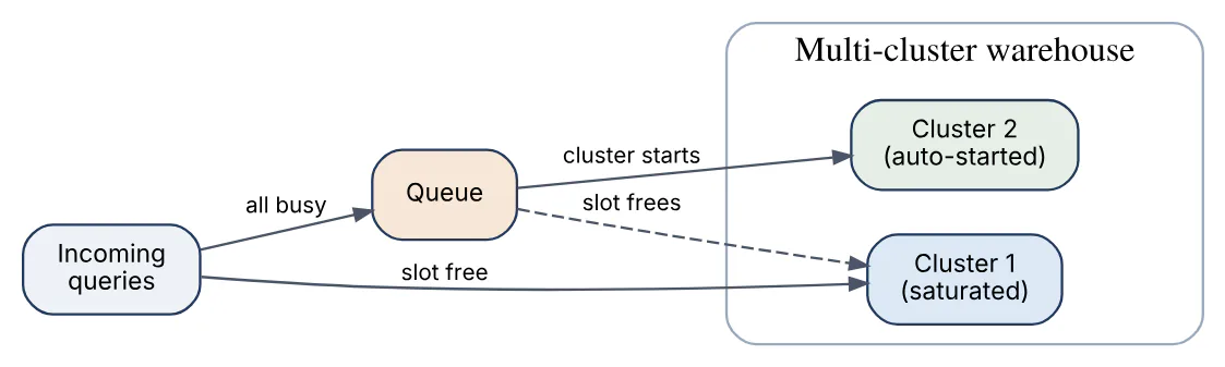
Ways to scale it:
- Multi-cluster warehouses (Enterprise and above) add whole clusters between
MIN_CLUSTER_COUNTandMAX_CLUSTER_COUNT; theSTANDARDpolicy favours starting clusters to avoid queuing,ECONOMYfavours keeping clusters busy. - Workload isolation with a warehouse per team or job type, so batch never queues BI.
- Larger size speeds each query, which frees slots sooner, but does not add parallel capacity the way clusters do.
- Query Acceleration Service offloads parts of large scans to shared serverless compute.
- Caching through the result cache (24 hours, free) and the warehouse SSD cache makes repeated BI queries almost free.
In BigQuery, concurrency is governed by slots: on-demand shares up to about 2,000 slots per project, editions autoscale slots, and queries queue only when capacity is exhausted; a per-project concurrent-query limit also applies when queries are interactive. The Snowflake fix is more clusters, the BigQuery fix is a higher autoscale maximum or a dedicated reservation.
74In a real project using Snowflake / BigQuery, how would you apply, test, or troubleshoot warehouse concurrency performance?
Apply. A retail BI platform served 600 store managers who all open the same dashboards at 8 a.m. I put them on a dedicated multi-cluster BI_WH (size M, 1 to 6 clusters, STANDARD policy, five-minute auto-suspend) separate from ETL and data science warehouses. Dashboard queries were made cache-friendly by removing CURRENT_TIMESTAMP() from the SQL so identical requests hit the result cache.
Test. Before launch I replayed a captured hour of dashboard traffic at 3x speed with JMeter against a clone of production data and recorded p95 latency and the maximum cluster count reached. The acceptance rule was p95 under four seconds with no query queued longer than five seconds; the run showed that a cap of four clusters was insufficient, so the maximum went to six. Afterward, WAREHOUSE_LOAD_HISTORY is reviewed weekly.
SELECT warehouse_name, DATE_TRUNC('hour', start_time) AS hr,
       AVG(avg_running) AS running, AVG(avg_queued_load) AS queued
FROM   snowflake.account_usage.warehouse_load_history
WHERE  warehouse_name = 'BI_WH'
GROUP  BY 1, 2 HAVING AVG(avg_queued_load) > 0.5 ORDER BY 2;
Troubleshoot. Users reported spinning dashboards at 8:05 although the warehouse was multi-cluster. History showed MAX_CLUSTER_COUNT had been lowered to 2 as a cost measure, and clusters take a minute to start, so queuing peaked before they came online; raising MIN_CLUSTER_COUNT to 2 during business hours with a scheduled task removed the spike. If queued_provisioning_time is high, startup is the issue; if single queries are slow with no queuing, resize instead.
More clusters multiply cost linearly and do nothing for one slow query, so diagnose queuing versus slow execution first.
75Explain pipeline idempotency in the context of Snowflake / BigQuery.
A pipeline is idempotent when running it more than once for the same input, because of a retry, a backfill or a duplicate trigger, leaves the target in exactly the same state as running it once. It matters because orchestrators retry, message brokers deliver at least once, and operators rerun jobs after incidents.
Techniques that work in both warehouses:
- Overwrite by partition — rewrite one date slice completely (
INSERT OVERWRITEin Snowflake,WRITE_TRUNCATEto a partition decorator in BigQuery) rather than appending. MERGEon a business key — upsert so a repeated row updates itself instead of duplicating.- Deduplicate on read or load —
QUALIFY ROW_NUMBER() OVER (PARTITION BY key ORDER BY ts DESC) = 1. - Deterministic inputs — parameterise by run date, never
CURRENT_DATE, and use deterministic surrogate keys (hashes) instead of sequences or UUIDs generated at runtime. - Load tracking — Snowflake
COPY INTOremembers loaded files for 64 days and Snowpipe for 14 days; BigQuery load jobs accept a client-suppliedjobId, so a resubmitted job with the same ID is not executed twice. - Atomic publish — build in a staging table, then swap (
ALTER TABLE ... SWAP WITH, orCREATE OR REPLACEfrom a snapshot).
MERGE INTO curated.orders t
USING (SELECT * FROM staging.orders_batch
       QUALIFY ROW_NUMBER() OVER (PARTITION BY order_id
                                  ORDER BY updated_at DESC) = 1) s
ON t.order_id = s.order_id
WHEN MATCHED AND s.updated_at > t.updated_at THEN UPDATE SET *
WHEN NOT MATCHED THEN INSERT *;
Plain INSERT of a batch, and any logic depending on CURRENT_TIMESTAMP(), are the usual idempotency breakers.
76In a real project using Snowflake / BigQuery, how would you apply, test, or troubleshoot pipeline idempotency?
Apply. In a payments pipeline on Airflow, each task receives a logical date and rewrites exactly that slice. Raw loads use COPY INTO with its file tracking; the transformation deletes and reinserts the day’s rows inside one transaction (Snowflake) or overwrites a single partition (BigQuery), and the final merge into the reporting table keys on transaction_id. Surrogate keys are MD5(transaction_id || source_system), so reruns generate identical keys. Retries are therefore enabled on every task without fear.
Test. The key test is run-twice-and-diff: in CI, the pipeline runs for a fixed day against fixtures, a checksum of every output table is captured, the same day is run again, and the checksums must match. A second test replays a batch with 10% duplicated rows and asserts the output row count equals the distinct input count. A third kills the task mid-run, reruns it, and checks for partial leftovers. Late-arriving data is covered by running a day, adding a corrected record, and rerunning.
Troubleshoot. Duplicates appeared in the daily revenue table after an Airflow retry. The task did INSERT INTO ... SELECT and failed after the insert but before acknowledging, so the retry inserted twice. Converting it to a MERGE fixed it, and a uniqueness test on the business key now guards the table. Another incident: a backfill produced different numbers than the original run because a model used CURRENT_DATE to compute “age in days”; passing the logical date as a variable made it reproducible.
Idempotency covers the warehouse writes; side effects such as emails or API calls outside the warehouse need their own deduplication keys.
77Explain cross-cloud data movement in the context of Snowflake / BigQuery.
Cross-cloud data movement is transferring or exposing data across cloud providers or regions, for example from AWS to Google Cloud. It is constrained by egress charges, latency and governance, so the choice is between moving data, replicating it and querying it in place.
Options on Snowflake:
- Database and account replication (
ALTER DATABASE ... ENABLE REPLICATION TO ACCOUNTS, replication and failover groups) copies data to accounts in other regions or clouds, refreshed on a schedule; this is also the foundation for cross-region sharing and disaster recovery. Egress is billed for the transferred bytes. - Cross-cloud auto-fulfillment for listings replicates shared data to consumer regions automatically.
- External stages and
COPY INTO <location>unload to object storage in any cloud for file-based exchange. - Iceberg tables with an external catalog let engines on different clouds read one open-format copy.
Options on BigQuery:
- BigQuery Omni runs queries against data in S3 or Azure Blob without moving it, and cross-cloud transfer (
CREATE TABLE AS SELECTorLOAD DATAfrom Omni to a Google region) moves results. - Storage Transfer Service and the BigQuery Data Transfer Service copy files and tables from S3, Azure and other sources.
- Cross-region dataset replication and managed disaster recovery for editions replicate within Google Cloud.
The guiding principle is to move the smallest thing that answers the question: aggregated results rather than raw tables, and incremental changes rather than full copies. Egress, typically a few cents per GB, dominates cost for large volumes.
78In a real project using Snowflake / BigQuery, how would you apply, test, or troubleshoot cross-cloud data movement?
Apply. A company with its core platform on AWS and its machine-learning team on Google Cloud needed daily features in BigQuery. Rather than copy the 8 TB fact table nightly, I aggregated features inside Snowflake into a 40 GB table, unloaded it as Parquet to S3 with COPY INTO @stage, and used BigQuery Data Transfer Service to load it into a partitioned table each morning. For disaster recovery, a Snowflake failover group replicates the curated database to a second region on a 30-minute schedule.
Test. Completeness is verified with a manifest: the unload job writes row counts and per-file checksums, and the BigQuery load job’s row count must equal the manifest total or the pipeline fails. Replication is tested by promoting the secondary in a drill, running the top reports against it, and measuring the recovery point from REPLICATION_GROUP_REFRESH_HISTORY. Cost is tested by estimating egress from bytes unloaded before the first production run.
Troubleshoot. The transfer started taking five hours instead of one because the unload produced ten thousand tiny files; setting MAX_FILE_SIZE to about 250 MB fixed throughput. An unexpected bill came from replication of a table with frequent full rewrites, since every refresh shipped the changed micro-partitions; moving it out of the replication group and rebuilding it in the secondary from replicated sources removed the cost. Type mismatches (Snowflake NUMBER(38,0) versus BigQuery NUMERIC limits, timezone-aware timestamps) surfaced as load errors and are handled by explicit casts in the unload query.
Compliance often limits movement more than cost does: data residency rules may forbid copying certain datasets out of a region at all.
79Explain production incidents and recovery in the context of Snowflake / BigQuery.
A production incident is any event that makes data wrong, late or unavailable: a bad deployment, a failed load, a runaway query bill, an accidental drop, a permission change that blocks users, or a platform outage. Recovery means restoring correct service quickly, then fixing the cause and preventing recurrence. The tools differ by failure type:
| Failure | Snowflake recovery | BigQuery recovery |
|---|---|---|
| Dropped or overwritten table | UNDROP, Time Travel clone (up to 90 days) | Time travel copy (2 to 7 days), snapshot |
| Bad data loaded | Clone BEFORE (STATEMENT => id), rerun | Restore snapshot, rerun idempotent job |
| Regional or account outage | Replication and failover groups | Cross-region replication (editions) |
| Runaway cost | Resource monitor suspends warehouse | Slot cap, maximum_bytes_billed, quotas |
| Leaked credentials or bad grant | Disable user, rotate keys, revoke role | Revoke IAM binding, audit logs |
Good recovery depends on preparation: a defined RPO and RTO per dataset, backups that exercise the restore path, runbooks, alerting on freshness and volume rather than only on job failure, and blameless post-incident reviews. Fail-safe in Snowflake and the 7-day fail-safe in BigQuery are last resorts reachable only through vendor support.
Query history (QUERY_HISTORY, INFORMATION_SCHEMA.JOBS) and audit logs are the first diagnostic sources, since they show who ran what, when, and with which resources. Snowflake’s status page and Google Cloud’s status dashboard separate platform incidents from your own.
80In a real project using Snowflake / BigQuery, how would you apply, test, or troubleshoot production incidents and recovery?
Apply. For a revenue-critical warehouse, I classify datasets into tiers: tier 1 has a 15-minute RPO and one-hour RTO, with 30-day Time Travel (Snowflake) or daily snapshots plus seven-day time travel (BigQuery), cross-region replication, and freshness alerts. Every pipeline records its query_id or job ID per run, so a bad run can be reverted precisely. Runbooks exist for the common cases: restore a table, roll back a release, kill a runaway query, rotate a service credential. Deployments happen through CI with a pre-deploy clone or snapshot.
Test. Recovery is only real if rehearsed. Each quarter a game day drops a tier-1 table in a staging account and times the restore against the RTO, fails over to the secondary region and runs smoke queries, and revokes a service account’s role to confirm alerts fire and the runbook is accurate. Alerts are verified by deliberately delaying a load and confirming the freshness monitor pages within its threshold.
Troubleshoot. In one incident a deployment overwrote a fact table with a join that dropped 12% of rows; dashboards showed a revenue dip. Diagnosis: freshness was fine but the row-count monitor flagged the drop, QUERY_HISTORY identified the statement, and the table was restored with CREATE OR REPLACE TABLE ... CLONE ... BEFORE (STATEMENT => ...) within minutes, followed by a fixed release and a new row-count assertion in CI. In another, a looping BI refresh burned a month of credits in a night; the resource monitor suspended the warehouse at its quota and the blast radius was one team’s allocation.
Time Travel and snapshots restore data but not the damage downstream, so lineage is needed to find and rebuild every dependent table and notify consumers.
Answers tailored to your resume and job description
Add your resume and the job description in CrackItX's Settings. When the interviewer asks a Snowflake / BigQuery question, Claude suggests an answer using your real projects and the role's requirements, in real time.
See pricing →